Chapter
1. Interface of Mathcad (of the book «Mathcad 12 for Students and Engineers»)
See All
Figs, WorkSheets and WebSheets >>>>>>>
Table of Content:
1.2. VFO
(Variable-Function-Operator)
1.4. Calculation with physical
quantities: problems and solutions
1.5. Three dimensions of Mathcad
worksheets
1.7. Animation and pseudo-animation
Mcd-
files and MAS/MCS WebSheets - >>>>>>>
1.1. Input/displaying
of data
This is a
general way to solve a problem in Mathcad: a user usually types the (new)
source data and some operators to work it out in the worksheet, or uses his own
or other ready-made procedures[1]
and obtains a result. This chapter contains not only some descriptions of the
instruments for input/displaying information but also a review of their
development and their critical analysis.
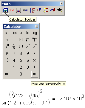
When Mathcad
appeared on the market of computation tools, it was advertised as, and was
called a super calculator: if one
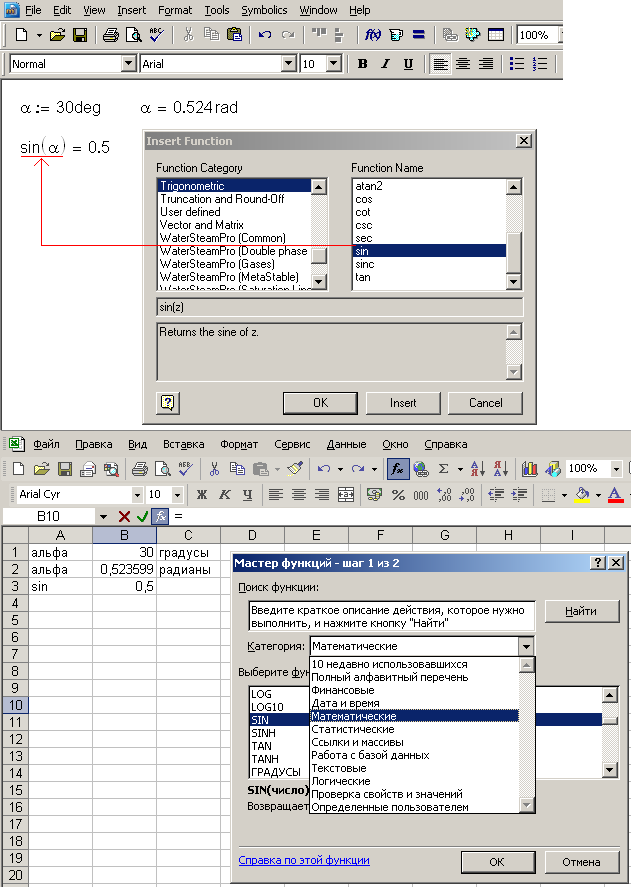
clicks = (the evaluation equal sign) after an expression Mathcad shows the result (Fig. 1.1).
Comment
The equal sign is the
usual “thin” equal sign located on the upper-right corner of the keyboard.
There is also a “bold” equal sign of equality, Boolean equality, inserted by
clicking the keystroke <Ctrl>+<=> or by the corresponding button
from the Boolean toolbar. A novice user
often confuses these operators and presses <Ctrl>+<=> instead of
<=> or vice versa, that is, in turn, tangles the calculation. There was
no such confusion in the DOS-versions of Mathcad. Keystroke <Ctrl>+<=
displayed not a “bold” equal sign but a wavy line; a half of an appro
The term
“super calculator” remains partly in Mathcad in the name of the toolbar[2]
Calculator (see Fig. 1.1). This
contains the basic mathematical functions and operators as well as the operator
= (the latter showing as Evaluate Numerically when the mouse pointer hovers over the button). This toolbar actually
copies the keyboard of the “scientific” calculator[3], the real one or virtual,
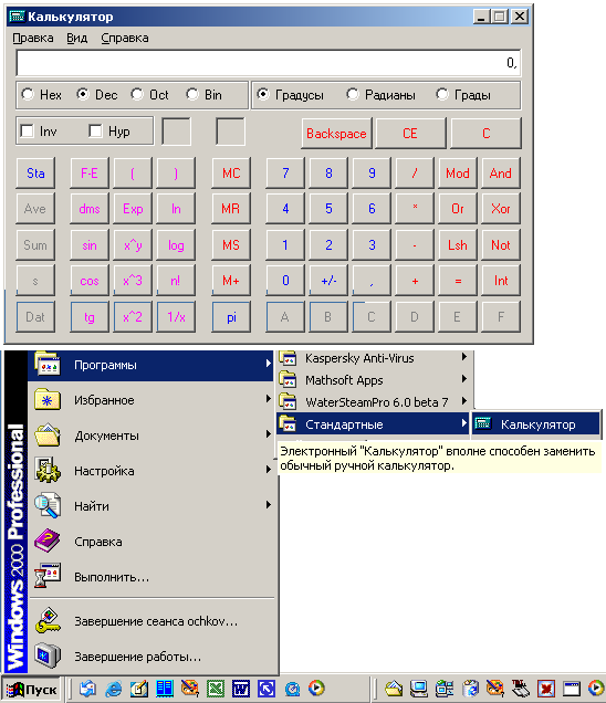
for example, such as contained in Windows. Fig. 1.2 shows the so-called
scientific calculator, and the commands to call it in one Windows version.
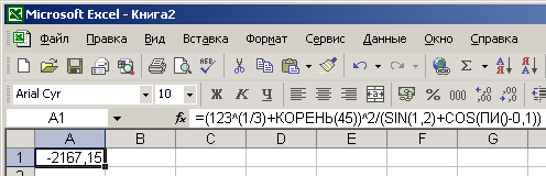
The equals
sign = has the same evaluation effect in another popular calculation
environment, the electronic worksheet MS Excel.[4]
However, there it is placed not at the end of a mathematical expression as in
Mathcad (see Fig. 1.1), but at the beginning (Fig. 1.3).
Both in
Mathcad and in MS Excel the numerical result is displayed just after
typing a formula and pressing the Enter key (automatic mode set by default) or
after pressing <F9> key (automatic and manual modes). MS Excel shows
the result in the cell contained the corresponding formula (cell A1 in Fig. 1.3) substituting for
the formula itself. Therefore, we cannot see simultaneously both all the
formulae and its results. In Mathcad, the result is placed to the right of a
formula and does not cover it.
Comment
Mathcad has a mode
which shows the result of an analytic conversion in the place of the source
expression. The problem of whether to show simultaneously both the formula and
its result or to do it in turn is connected with, first, saving the spare place
on a screen and paper of a printer and, second the aim of calculation, its
direction. If the aim of a calculation is mere practice, working out new data
and showing a result, the formula would be unnecessary. If the study of the
calculation is necessary for educational purposes, additional checking of the
result, or making some changes, the formulae would not be excessive. Mathcad
has the instruments to hide the formulas, which will be discussed further.
We will
note straight away that the calculator in Mathcad (Fig. 1.1) differs from
other similar calculation systems (See Fig. 1.2 and 1.3). It can work both
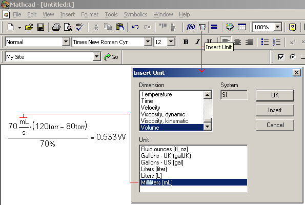
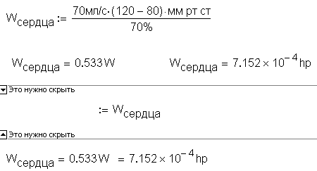
with figures and with physical quantities. Figure 1.4 shows the Mathcad calculation of the
power of a human heart having the following parameters: it pumps 70 ml of blood
per minute (mean statistic of a man at rest), the pressure increases from 80 to
120 torr, and efficiency of this living pump equals 70%.
Mathcad
has built-in units for basic physical quantities as well as fundamental
mathematical constants, such as e (the radix of natural logarithm) or p (ratio of circumference to its
diameter), etc. A detailed description of this Mathcad feature will be given in
sec. 1.4. Mathcad also has a
quite thorough reference book containing basic mathematical, physical, and
chemical constants, which can be copied into a worksheet with corresponding
units. For example, Fig. 1.5 shows how the calculation of the well-known
Einstein formula E=mc2 could be made in Mathcad, taking velocity of light in a
vacuum from the Reference book[5].
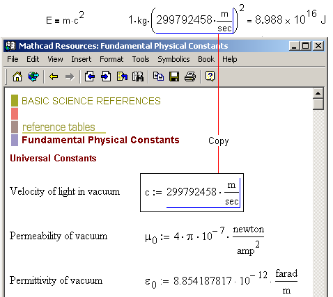
Figure
3.1 from ch. 3 shows that we
transferred not just a constant but the mathematical formula for a cone volume
calculation from the Reference book into the worksheet. The Reference book is
accessed by clicking Reference Tables from Help menu.
There are
two other principal differences between Mathcad and Excel.
The
formulae in Excel are typed in one string
and the mathematical operators are written in “programmer” form: for example, x^2 instead of x2 etc. This notation has such an excess
of parenthesis so that only a computer but not a man[6] can read rather long formula. For example, it is sometimes difficult to
understand where the nominator or the denominator is. A formula in Mathcad
follows a “many-storied” natural format.
There is a second
considerable difference. The worksheet in Excel is divided into columns and
lines at the intersection of which can be entered required information,
numbers, test, formulas etc. The Mathcad worksheet is a “clean paper” where we
can type anything anywhere. In addition, there is a possibility to insert
information in table format (see Fig. 1.18 and 1.20).
The Evaluate Numerically operator presents its evaluation
using a set of defaults that can be modified by clicking Result from Format menu
or double-clicking the result itself. Figure 1.6 shows two inlays of the
dialog box for formatting a numerical result.
The
following is a list of numerical evaluation defaults, far from complete, which
also evolved through the Mathcad versions.
r
The
numerical result is displayed as decimal but not as binary, octal, or
hexadecimal[7]. We can change the setting
via Radix from the Display Options tab shown in
Fig. 1.6;
r
The
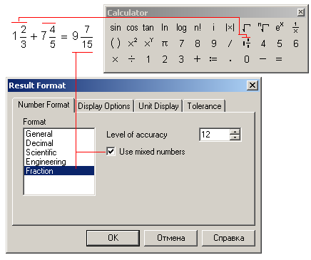
numbers are displayed as decimal fractions (for example, 1.333) but not vulgar
(4/3 or 1 ⅓) although that is possible in Mathcad too (choose Fraction
from the Format list in
the Number Format tab
as Fig. 1.6 shows);
Comment
Inserting a number
as vulgar fraction is possible through normal addition or division (for
example, а:=1+1/3)
or, if one prefers omitting the plus sign, by clicking ![]() on the Calculator toolbar.
on the Calculator toolbar.
r
Only three numbers are displayed after point (Number of decimal places from the Number
Format tab in Fig. 1.6);
r
The number is displayed in exponential notation as it is less than 10–2 (Exponential threshold from the Number Format tab in
Fig. 1.6);
r
If the fractional part of a number ends in zeros they are not displayed
(Show trailing zeros from the Number Format tab in Fig. 1.6);
r
the number is appro
r
the imaginary unit of a complex number is marked as i but not j
r
the background is white and the numbers are black etc[8]
Mathcad users can
both change these defaults formatting the current result and change the
worksheet default. After changing the settings, click Set as Default in the Number Format tab from the Result Format
dialog box.
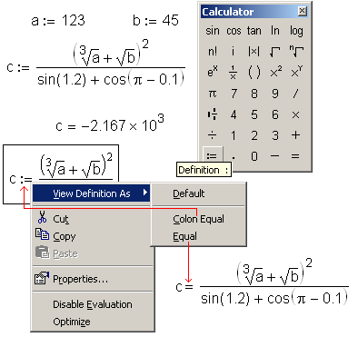
The second most important operator is the assignment (definition) marked as :=. To enter it just press <:> (colon). Mathcad
courteously adds the second sign (=) moving the cursor to placeholder
for entering a number or an expression. For example, Fig. 1.7 shows
insertion of three user variables, a, b, and c, two of which (a and b) are the
source data, and the third is defined as the result of the calculation by the
formula.
Comment
Another way to enter the assignment sign in Mathcad is
to click the corresponding button on the toolbar (for example, see left bottom
corner on the Calculator toolbar in Fig. 1.1). The
third way is to copy and paste the assignment operator entered before. In Mathcad
any operation can usually be done at least three ways.
Starting
with the seventh version users have the capability to change the definition
sign from := (style of the Pascal language) to = (BASIC[9]). The pop-up menu for changing the view of the definition operator is
called by clicking on the operator with the right mouse button. Fig. 1.7 shows that it has three
positions: Default, Colon Equal, and Equal. Although, if the pointer is placed on the
expression which the assignment sign was changed from
:= to = the previous default symbol:= is returned. The users seldom
substitute the = sign for := since it results in confusion: for example:
a = 1 a = 1 What is this?
The notation
a:=1 a=1
is quite clear.
The operator :=
should be called more precisely the
half-global assignment because we can compute with the function defined by
the operator anywhere to the right and below of the expression that defines it.
Comment
The variables in the calculation are sure signs that
distinguish programming from simple calculating ― compare calculations on
the Fig. 1.1 and 1.7. The variables in Mathcad are discussed in section 1.2.
Comment
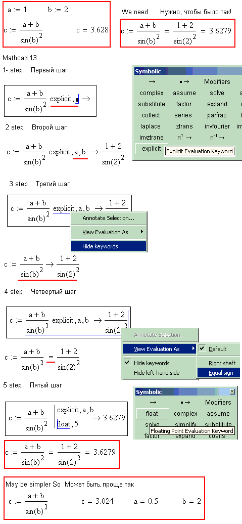
Here is a typical
mistake made by a novice Mathcad user. The horizontal chain of operators is
entered:
A := 1 b := 2 c := a + b
The third operator
is interrupted by the error message “Variable is not defined”. An operator
located a little higher than the others may be imperceptible to your eyes but
will interrupt the calculation. To avoid such errors the recommended practice
is to type the operators in columns pressing <Enter> after
each expression. To make worksheets more compact we can use the second
dimension in a finished worksheet, locating some operators in lines. It is also
possible to have the third
dimension in Mathcad (see section 1.5).
The
symbol for the global assignment operator is ≡. We introduce it by typing
<~> or by clicking on the corresponding button on the Evaluation toolbar. The scope of the variables
and functions defined by it is the entire Mathcad worksheet; it spreads from
operator ≡ wherever one wishes.
However, using this operator is not highly recommended; it breaks cause-effect
relation and confuses those who aim to study the document: a variable has a
defined value but is not clear where it was defined. Moreover, this operator
can define only constants (for example a≡3, the operator is sometimes called
the operator of constant definition), but not the expressions containing other
constants (for example, a≡2b). Some users define the variables that change
the values in calculation using the operator := (for example, from a:=1 to a:=2) and the variables that do not change using
the operator ≡.
This users fail to take into consideration the difference in scope. Although,
the global assignment operator can influence to top of the worksheet, for
example, damage plots created by QuickPlot. Separating assignment operators ![]() := constant from
:= constant from ![]() ≡ constant can be useful before the key word Given. Thus we comment that some variables
are constants, while others are the first appro
≡ constant can be useful before the key word Given. Thus we comment that some variables
are constants, while others are the first appro
Mathcad
can solve problems numerically
(approximately) as well as analytically
(symbolically). The symbolic equality operator is ®.
It will be discussed below.
As
Fig. 1.8 shows the interface operators described above =, :=, ≡, and ® are collected (some of them are duplicated) in
the distinct panel Evaluation. Section 1.2 deals with the other
buttons in this panel.
Mathcad
also has a local assignment operator. Operator ¬ makes the variables defined only within a
Mathcad-program. Chapter 6 will have
more about that operator.
Comment
Both operators ¬ and ≡
can be changed to the more customary = . Fig. 1.7 outlines how to do it.
By means
of the very convenient built-in feature, Style
of variables, Mathcad allows distinct variables to have the same textual
name. By default, the variable introduced into a worksheet is assigned the
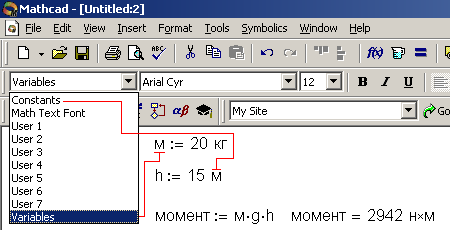
style Variables (Fig. 1.9).
A Mathcad
user can change the style of a variable and insert a new variable with the same
name into a worksheet. Fig. 1.9 shows this feature of Mathcad: a certain
moment of force, m, is calculated (the product of force (or, rather, weight — the product
of a mass m and acceleration of gravity g) and arm length of the force
application) using two variables of the same name. Speaking about the texts and
comments Mathcad offers a set of style for dealing with text regions (see sec. 1.3) allowing the user to
format letters, words, paragraphs (title of the first level, title of the
second level) practically as in MS Word.
Beginning
from the eighth version, Mathcad allows to enter the evaluation equal sign
typing not <:> but <=>. The point is: if the variable is not defined the operator = (displaying)
is changed automatically into :=
(definition). Otherwise, if the assigning variable has already been defined its
numerical value is represented. So, one can check that the name is free: neither a user nor Mathcad has
defined it yet. Such technique allows us to omit a number of errors mentioned
before. First, some predetermined
variables could be changed: е:=5, m:=1, A:=2 etc. Variable e is the radix of the natural logarithm and variables m and A are units of length (meter) and current
strength (Ampere) accordingly — see Fig. 1.9. Second, one could forget
that a user has already defined the variable and assign it something new. The
situation when the same variable has one value in the first part of Mathcad
worksheet and another in the second part is not right.
The
technique of variable redefinition is used when the memory was a limiting
parameter in computing so that the spare variable was redefined right away to
omit memory overflow.
Comment
In Mathcad the
variable keeping a massive (vector or matrix) can include text, scalar (real or
complex number) and vice versa. A variable in Mathcad is not connected with one
or another variable type that exists in most part of traditional programming
languages.
We use
such technique now in locating the extensional arrays (vectors and matrixes, simple and compounded) in computer
memory (including that working with Mathcad). Although, redefining the new smaller
array or ever a scalar value does not change the volume of memory (the
mechanism of static arrays but not that dynamic).
Comment
Besides, this
technique is not applicable to arrays. If one types V in a
spare Mathcad worksheet [0 and pushes the button <=> to
enter zero element (constant) of vector v Mathcad displays an error message
instead of equal sign.
The mode
of automatic change of assignment operator from = to := (such a hybrid of two
operators called SmartOperator [10])is
disabled by throwing of a flag from Context-sensitive equal sings of the
General tab from the Preferences dialog box calling by the same command from the Tools or Math
menu in Mathcad 2001i and in earlier versions (see Fig. 1.10).
Fig. 1.10
shows a very interesting and useful number
At a
certain stage of Mathcad development it becomes possible to enter some
interface operators in tandem,
feeding one input/display operator into another. Thus, point 1 of
Fig. 1.11 shows the use of the operators ® and = (symbol and numerical result) in solving the
equation. The advantage of a symbolic result is absolute accuracy and numeric
shows the distinct location on the number axis (or on a plane in the case of
complex number). The tandem use of operators allows us to combine those
advantages.
Comment
Including one
operator (one function) into another operator (function) on the place of
operand (argument) is a traditional programming method. But it is quite exotic
for input/display operators in Mathcad.
Fig. 1.11
at point 2 shows us the tandem operators at work. := and ® (Definition and Evaluate Symbolically) allow
us to enable symbol mathematics, for example, to create a user function or its
derivative. Those two useful tandems (points 1 and 2 in
Fig. 1.11) were in the category of undocumented techniques and later on
became kind of half-documented: they are not described in the product
documentation but are recommended for use in different sites Mathcad-supported
sites including the developer’s official site www.mathsoft.com. The
tandem of operators := and ®
is the same as Optimize mode from the pop-up menu shown in point
Still
undocumented is the tandem operators ¬ and ® ( local definition and symbolic equal sign,
see point 3 in Fig. 1.11) which enable us to look through the
variables in programs and is very useful in checkout. This feature is discussed
in Ch. 6.
The
evaluation equal sign became a stumbling block for those who started Mathcad
ten or fifteen years ago, hearing of its unusual abilities for calculating
sophisticated formulae (see Fig. 1.1), making graphs (see sec. 1.6), animations (see sec. 1.7), solving equations and
systems of equations (See Ch. 2).
Through a habit formed by working with Fortran or BASIC users typed a= in Mathcad instead of a:[11] and… refused to work with this mathematical
package further. An error, unintelligible at first glance, had emerged: Mathcad
informed them that a variable is not defined. Users tried to define that error
by operator of variable type being guided by experience of working with
programming languages, but Mathcad has not such operator. By the seventh
version Mathsoft company had “surrendered” and stopped demanding users to type а: instead of more convenient and customary a=. Now the pendulum has swung to the
opposite side: now to assign the value to a variable it is recommended to type a= rather then а:. We could recommended that Mathcad developers
excluded the operator := at all but it is necessary for changing the value of predetermined
variables (for example, TOL:=10–7, ORIGIN:=1) and for defining a user function or an
element of a vector. Although, even in these cases one can omit operator := coping it from the place where it
was created by “smart” operator =.
It is
also advisable to use the equal sign for evaluation for defining a user function in Mathcad. After typing
the name of a new function it is better to press not <(> ( a parenthesis opened a list of
arguments) but <=>. The reason is the same: to protect a user from the
possible errors connected with reassignment of the functions. For example, if a
user want to insert a function named F and types couple of symbols F= Mathcad may display the following:
r
F = 1 F the unit mode is not disabled. In
this case, Mathcad remind us that farad (unit of electrical capacity) equals to
1 farad and this variable name is occupied.
r
F = number means that the user variable with
name F already
exists in the worksheet.
r
F = function means the user function with name F already exists in the
calculation.
Comment
In Mathcad 12 the word function now appears in
brackets: F=[function].
r
F := — means that the name is spare and
available for use as a function or a variable name.
There is another
variant: if the name of planning function coincides with that of the built-in
function after pressing <=> it will be duplicated, for example line = line. The Mathcad user should decide
what to do in this situation. In some cases, reassignment of a function solves
certain difficulties of calculation.
Comment
The name will be
duplicated in mode of “early” Mathcad calculation mode. In the Higher Speed
Calculation mode Mathcad shows line = function. Besides,
Mathcad 12 has only “quick” mathematics.
Old
habits die hard: it is impossible to break Mathcad users of the habit of using operator
:= to define variables or functions and force them to use = which ,as we noted
before, automatically chooses what a user want of him : definition or
displaying. Because of it the users continue to make the errors mentioned above
in connection with reassignment of variables. Through it Mathcad 11.1
(Mathcad 11 was published and patch 11.1 was released soon after it)
provided the user with the mechanism for checking the reassignment of variables
and functions, built-in and users, opened and hidden in closed regions (see
Fig. 1.22) and in referenced documents (see Fig. 1.21). For this, the
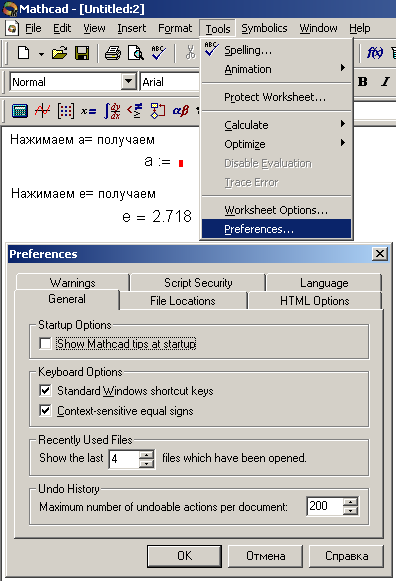
Preferences dialog box get the new Warnings tab (see Fig. 1.12).
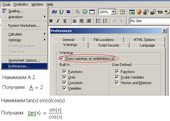
Developers
added a green wavy line to the Mathcad armory; in other environments, for
example, in Word it is used to mark incorrect punctuation. If such line appears
in a Mathcad worksheet under the name of assigned variable or defined function
the user should correct an error or just size up that something is out of order
here and knowingly reassign the variable and/or the function name.
Starting
with Mathcad 2001 the operator := assigns both the numerical values and text
literals, for example, c:=123 or c:="text", and uses visual programming standard controls: Check Box,
Radio Button, Push Button, Text Box, List
Box, and Slider shown in Fig. 1.13.
Comment
The command Control both inputs the data into the
worksheet and shows the result (Fig. 1.16 shows such an example).
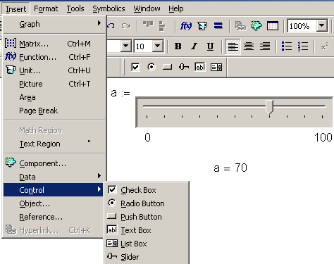
Controls
appeared in Mathcad to simplify the input of new data. Fig. 1.13 shows how
the value of the variable a is changed by simple mouse actions without any typing. At that, Mathcad
clearly shows the range of the variable (0—100), which cannot be overwritten by
a user by mistake or knowingly and the current location of the variable within
the range. The detailed description of these controls contains in
As the
need arose to have worksheets accessible by the Internet Mathcad acquired the
so-called Web Controls (See
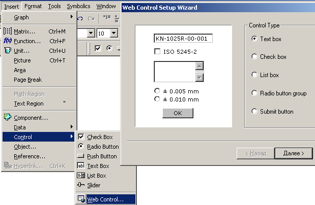
The
stages of preparing Mathcad worksheets for Internet publication are described
in details in
The
numerical evaluation operator has evolved too, or rather not the operator itself
but its function. Thus, current versions of Mathcad allow users to show numbers
also in non-decimal systems, both as vulgar and decimal fraction, in scientific
or in engineering formats, etc (see Fig. 1.6). However, operator = has not
got any distinct differences or additional format options apart from the cross
over with the operator := (SmartOperator, see Fig. 1.10). Such changes are
crucial from the standpoint of development of Mathcad Application Server (See
It would be so convenient if the numbers and texts
could appear and disappear without showing their sources: 123 and not b=123. When
showing text, it is desirable to hide inverted commas that frame it.
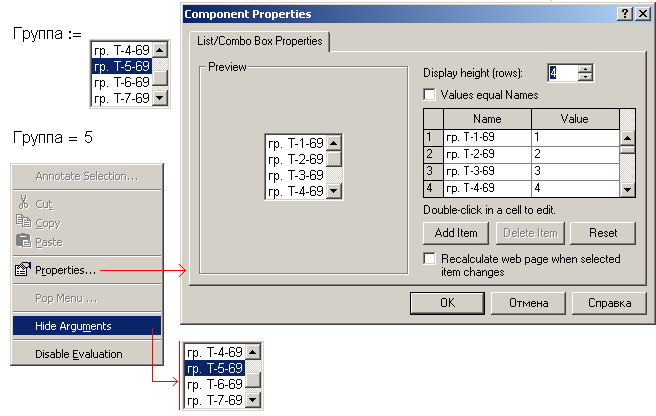
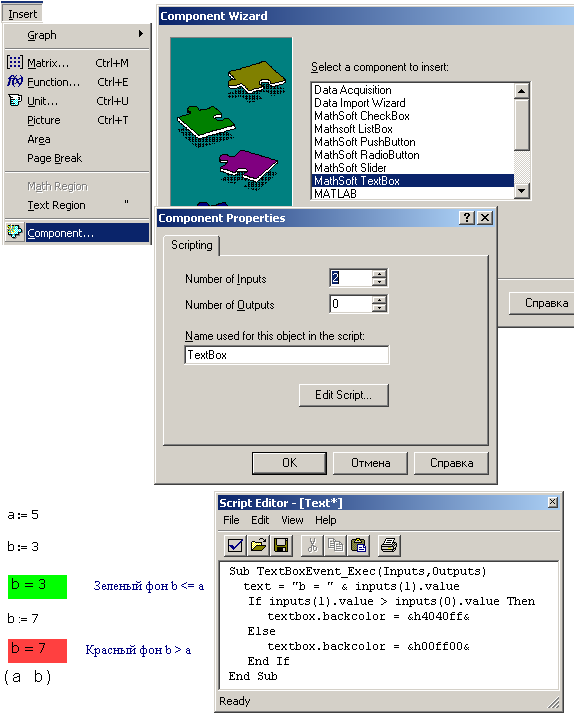
Also, it is desirable to change the format of
numeric and text literals (font, size, color etc) without using macros. For
example, Fig. 1.16 shows the way of changing highlight color of the
variable (operator b=) depending on its value by small macro
program. The macros are used to format Controls. As we noted before, Web Controls require simple
dialog boxes for formatting. Fig. 1.15 shows one of that used to format a
list; the other examples are contained in Ch.7.
Especially
we should take into consideration inserting the arrays (vectors and matrixes) into a worksheet, the data formatted
in rows and columns. This storage method is widely used both in paper
calculation and in computation.
The
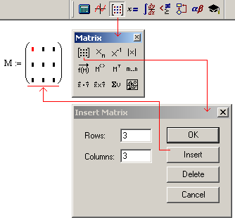
simplest method of inserting a matrix into a Mathcad worksheet is to choose Matrix from Insert menu, shown graphically in Fig. 1.17. However, it is
not very comfortable to enter numbers with the Matrix command. First,
we can insert at the most 100 array elements in such way. Through this limit
many of novice Mathcad users mistakenly think that 100 is the maximum number of
elements in a vector or matrix although user documentation said that it can
reach up to 8 million.
Comment
The vector (matrix
with one column) up to 50 elements is inserted simply by command v:=stack(element1, element2, ...). The built-in function stack turns the list of its arguments (which can be both vectors and
matrixes) into a vector.
It is more convenient to insert matrixes
via Insert | Data | Table as shown in Fig. 1.18. This command inserts the assignment operator ![]() :=
:= ![]() into the worksheet. Its right operand is rather bulky table (an analogue
of the Excel table); the user can type new information
in the its top left region forming the picture on the screen via the Component
Properties dialog box that also
shown in Fig. 1.18.
into the worksheet. Its right operand is rather bulky table (an analogue
of the Excel table); the user can type new information
in the its top left region forming the picture on the screen via the Component
Properties dialog box that also
shown in Fig. 1.18.
Comment
The earlier
Mathcad versions have “table” in the list of components (see Component in Fig. 1.18). Later on
this important component was located in a distinct menu item, Data, which contains two more commands
discussed below.
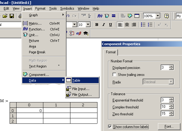
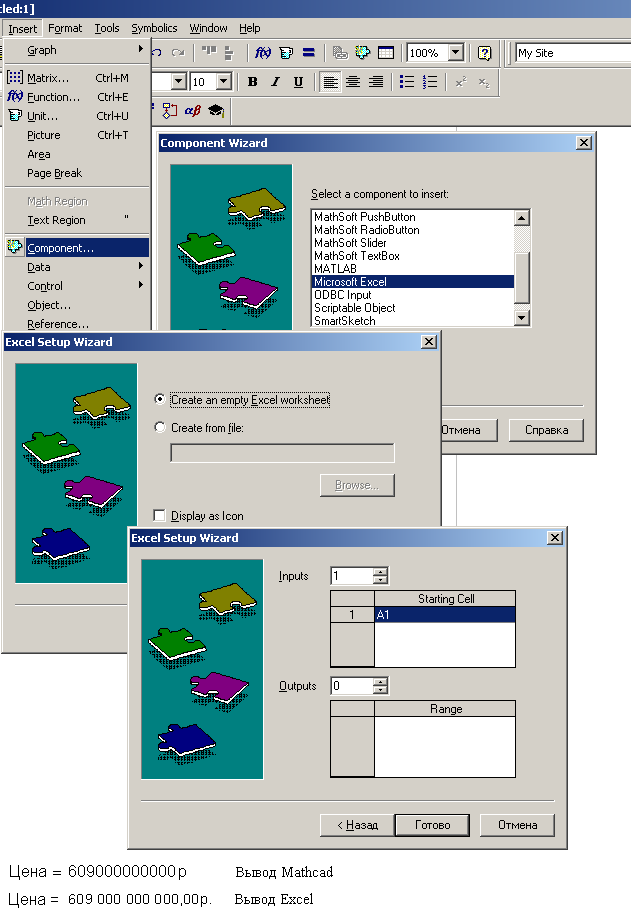
If a user
has installed both Excel and Mathcad, entering of large volumes of information
can be automated. An Excel table is inserted into Mathcad worksheet by choosing
Insert | Component... | Microsoft Excel and then in the Excel Setup
Wizard dialog box choose Create an empty Excel worksheet
or Create from file. After that we can point the part of Excel table
where the information from Mathcad is transferred (Inputs) or conversely
the information is transferred to Mathcad variable from Excel table (Outputs).
Fig. 1.19 shows that we “crushed a fly with a steam-roller” outputted
variable Cost in Excel using a special format of electronic
worksheet which inserts thousands spacer, white space between three numbers,
into numbers and thus, simplifying its reading. However, one can “crush”
earnestly, for example, to access those Excel functions that Mathcad does not
have (calendar functions) or to make Excel plot in Mathcad (pie chart).
Besides, to enter data in Excel table is more convenient and quicker: one can
use special Excel features –AutoFit and others. After entering data, the Excel
table can be removed to make Mathcad worksheet lighter, and in such case, and
so that those who have not installed Excel can work with the worksheet.
Beside Excel, one can insert other Windows
applications to Mathcad to expand its functionality and one can add Mathcad
worksheet into other applications, Word, for example. Nevertheless, it is only
worth inserting other programs into Mathcad worksheet if they provide
calculation and other features for which Mathcad is not sufficient. The point
is that the worksheet is sent to another user who does not have that application
the worksheet will fail. In addition, a Mathcad worksheet containing other
applications is difficult to publish on the Internet (See
Comment
To insert choose Object from Insert menu, common for all Windows applications.
Large
tables can be saved to disk as text files and connected to a Mathcad worksheet
by inserting the operators of writing/reading
a file to/from disk. Fig. 1.20 shows how to create the operator of writing
the data from file Tab_XV.dat and to send it to the variable M.
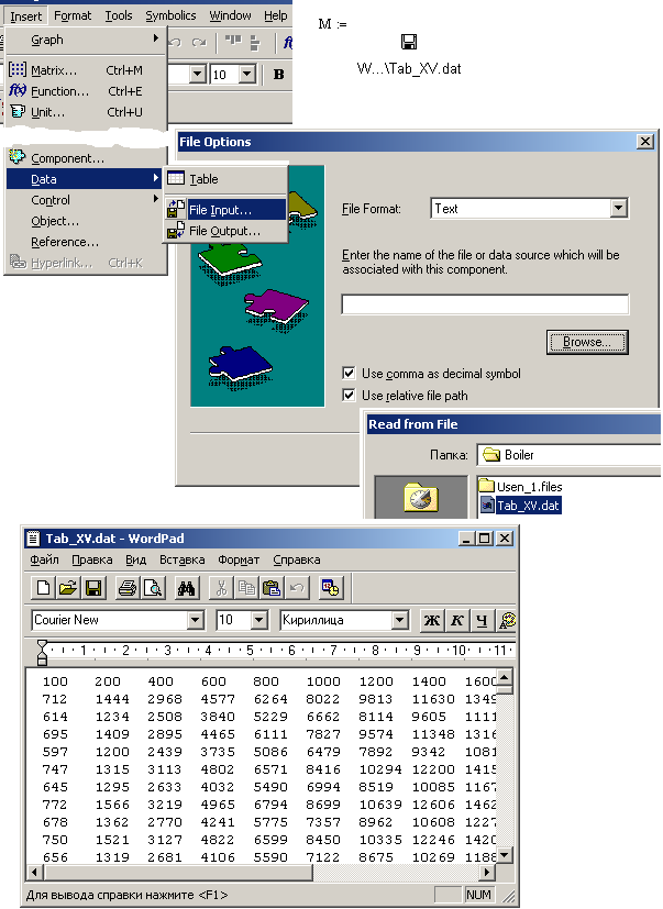
To assign
data to the variable M, choose Insert |
Data | File Input... that open
dialog box, or rather file changing wizard (File Options), in
which we can mark the file with required data in “file/disk/folder” Windows
system clicking button Browse of
the File Options dialog box. In addition, we can choose file format (in opening list File
Format) and set the the comma as
separator instead of the tab character. The data itself (Fig. 1.20 shows
it opening for review or editing in WordPad) can be entered in Mathcad and
written to the disk via command Insert | Data | File Output or
manually (for example, in Excel), or generated by another program, or received
by e-mail et cetera. Besides the command for data changing shown in Fig. 1.20
Mathcad has a set of similar functions (readprn, writeprn etc) accessed
by File Access from the Insert
Function dialog tab. The length
of numeric literal writing to disk depends on the value of built-in variable PRNPRECISION. The main disadvantage of saving
data in a file, rather than in Mathcad is that one can send Mathcad worksheet
and forget about the file[12].
To
exchange information between Mathcad worksheets choose Reference from Insert
menu.
It is not
necessary to contain all the operators for a given calculation within the
“current” Mathcad worksheet. They can be written in another worksheet, and
saved on a user disk or on any computer in local network. To make them work for
us, we must make a reference to the
file containing necessary data from the current worksheet. Fig. 1.21 shows
such situation. D disk contains Mathcad file sheet.mcd with address
D:\Documents and Settings\user\My documents keeping a single operator с:=a+b; of course, the calculating is interrupted by
an error message because the variables are not defined.
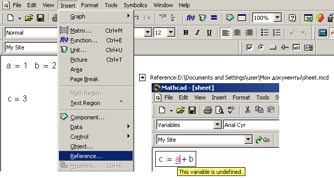
The other
Mathcad document which also shown in Fig. 1.21 contains operators of
source data (а:=1 b:=2) and the result (с=3). The worksheet named sheet.mcd carries out
the calculations contained in the referenced worksheet (which it is connected
to first by the command Insert | Reference). As a rule, the referenced documents
contains constants and functions covering a branch of applied sciences or having some general
engineering significance. With such references, we can make, for example,
dimensional a set of user functions in the form of DLL that were turned into
built-in i.e. listed in the Insert Function dialog box (see site www.wsp.ru).
One of the Mathcad’s interface features is the
ability to protect or to hide (a part of) the information.
As a rule, Mathcad worksheet comprises three parts: area for source data, area for calculation, and area for results. We can delineate
these areas in Mathcad worksheet clicking Area from the Insert
menu. This command insert two horizontal lines near the mouse pointer, after
which the user moves the top line to the start of an area they wish to create
and the bottom line to the end of their area (see the top of Fig. 1.22).
What can we do with it? First, we safeguard the information against unintended
edits by command Format | Area | Lock. After such command, the
region enclosed by the area can be viewed but not edited.
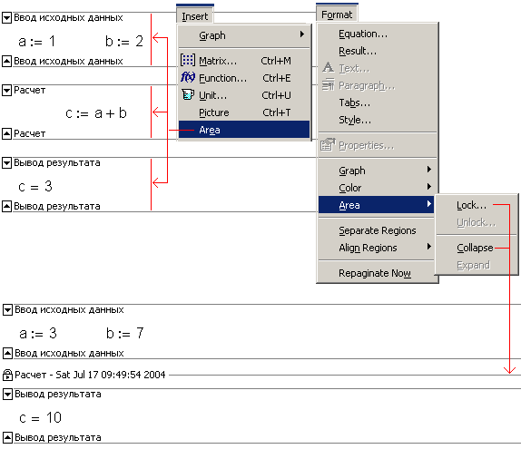
The second command used separately or together with
command Lock is Collapse and this hides the chosen area from a
user. The result of these two commands on the area named Calculation shown at the bottom of
Fig. 1.22. The user types this name clicking Properties from the
area pop-up menu. Otherwise, we can even hide a vestige of this area in Mathcad
worksheet by this command. After such manipulations (inserting, locking, and
collapsing an area) a user can change the values of a and b and see the result (variable c) but cannot see and edit the
formulae. A Mathcad worksheet containing a collapsed area is like a piece of
paper, the middle of which recedes into the background by several folds (
We can
safeguard Mathcad worksheet without inserting any areas, but safeguarding the
whole calculation while keeping some required operators unlocked.
Fig. 1.23 shows the menu commands allowing us to protect all, or the most
of, the worksheet.
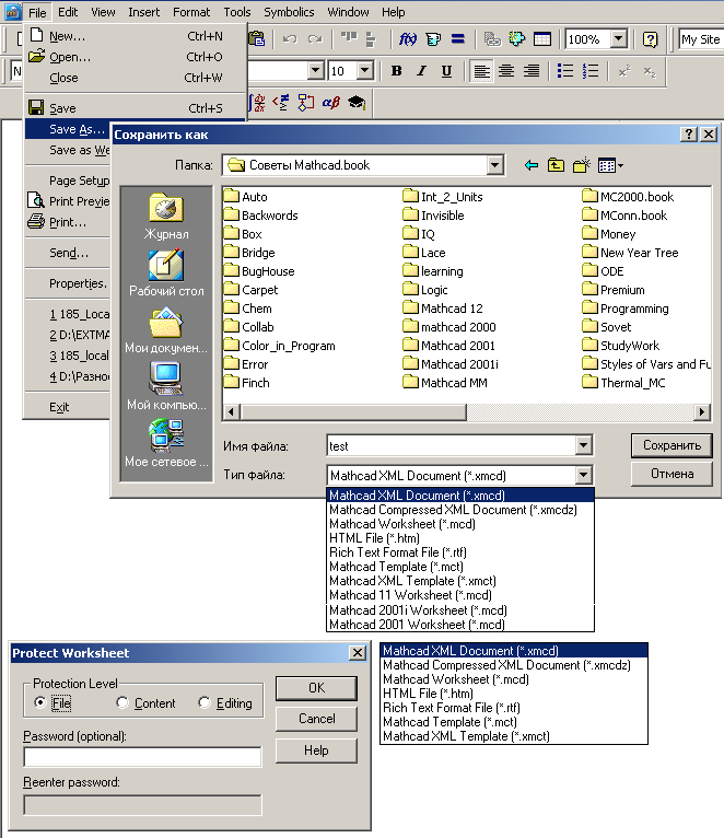
To protect
the worksheet, choose Protect Worksheet... from the Tools menu,
shown in the bottom part of Fig. 1.23. Worksheet protection comes in three
levels presented by switches Protection Level in the Protect Worksheet dialog box. The first level, File,
the lowest one, protect the worksheet from being saved in some formats, for
example as earlier Mathcad versions. Fig. 1.24 shows two lists of file
formats for saving the current worksheet even without protection level File.
In Mathcad 12 this protection level makes it impossible to save the
worksheet as Mathcad 11, 2000i, or 2000.
That
limitation works at two other levels too. The second level protects existing
operators against change by the switch Content
but new operators can be created. The third level, Editing, the highest one, does not allow us to change existing
operators or to create new. Of course, we can make the “holes” beforehand
i. e. turn off protection from some operators (as usual, from those defining
source information) by the commands shown at the top part of Fig. 1.23
with operator b:=7. In all levels we can protect the worksheet with a password or without
it (options Password (optional)
and Reenter password).
Some safeguarding mechanisms duplicate each other.
We can protect a separate operator or several operators at once placing them
into an area (Fig. 1.22) or by technique shown in Fig. 1.23[13].
This duplication occurs because the protection mechanisms were not introduced simultaneously but from earlier
versions to new. At the beginning, (Mathcad 2000) it became possible to
insert areas into worksheets (Fig. 1.22) safeguarding it against editing
only (Lock/Unlock). Then (Mathcad 2001) we could collapse these
areas (). Mathcad 2001i got the mechanisms
to protect whole worksheet and some of its operators (Fig. 1.23 and
1.24).
1.2.
VFO (Variable-Function-Operator)
The
previous section considered input/displaying operators ![]() =
= ![]()
![]() ,
, ![]() :=
:= ![]() ,
, ![]() ≡,
≡, ![]() ¬
¬ ![]() ,
, ![]() ®. This section will present what those
black squares calling placeholders may contain.
®. This section will present what those
black squares calling placeholders may contain.
1.2.1.
Function and operator
Mathematics
has a term correlation: for example,
there are two enumerable sets, and each element of the first correlates with a single element in the
second one[14]. The particular case of
such correlation is the one-argument
function y(x); for
example, any value of a angle (х is the first set and argument
of a function) correlates with value of sinus (y is the second set and the first function).
A middle-aged reader will get this right away well-knowing from Bradis tables
such “sets” of angles, sines, logarithms, and other necessary values. Of
course, Mathcad does not keep sets of angles[15],
sets of correspondent sines etc but calculates this trigonometric function in
accordance with its built-in algorithm. Another question is how accurate and
quick these algorithms are.
We may
note, for example, two sets of numbers, a set of functions and another set of
variables, and set of definite integral values: each four elements of the four
sets correlate with an element of the fifth set. The case in point is the
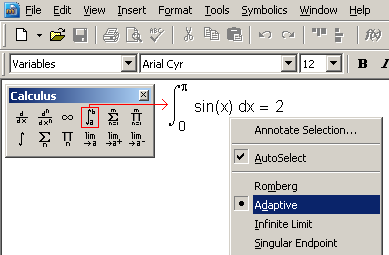
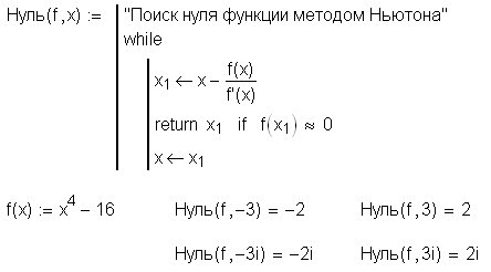
definite integral operator with four operands that is built in Mathcad
(Fig. 1.25)
About
thirty years ago, a discrepancy appeared between mathematicians and programmers
in terms “function” and “operator”.
A
mathematician reading this book may justly conclude that the author does not
fully understand what an operator is and what a function is. Moreover, there is
no unity of treatment of these terms in programming. “Operator” in Mathcad has
another meaning in BASIC, for example, and vice versa. Thus, BASIC has a
convenient operator Swap(a, b) that changes values of the variables a and b: c = a : a = : b = c, but without enabling variable c.
Comment
This operator
would not be superfluous in Mathcad, either. However, it would upset a stable
system functions and operators as it does not return a value but executes a
certain procedure.
As this
operator does not return a value, it cannot be called operator from the point
of view of a Mathcad user. On the other hand, Mathcad operators and functions
themselves may not return values either (for example the equality a=sin(x)) but be a peculiar comment (see sec. 1.3) and expect to be treated.
Comment
Besides, function sin of the operator a:=sin(x), for example, does not return a
value too. It will return sine of x if the operator a= appeares after the assignment operator.
Let us
agree that terms “operator” and “function” are application dependent and will
discuss not their essence (let the theorists dispute about it) but their
differences in Mathcad.
If terms
“operator” and “function” are considered in respect of the mathematics that we use
in calculations but not in respect of Mathcad features (see below about that)
we can mark out some aspects dividing Mathcad mathematical mechanisms into
operators and functions.
r A definite function is distinguished
from others by its name sin(х), cos(х), log(х). Operators differ from each other
by symbols n!, ¬x, ׀x׀, ò (see Fig 1.25) etc. Mathcad has
three operators with invisible (absent) symbol: xy (power), Xn (element of array or
text index), and 2K (multiplication). The visible operators will be
discussed in sec. 1.2.3.
r
Some Mathcad operators have ambivalent contents. For example, х2 what is it? Is it an operator with two power
operands, with the second operand equals to two, or squaring operator with one
operand? The second example: 2K is it a multiplication operator or just a variable named 2K (a name of this type is possible in Mathcad,
see sec. 1.2.2) etc. Mathcad
also has mathematical operations executed both as operators and as functions.
For example, the exponent is calling as ex (operator) and as exp(x)
(function). Basically, it would be convenient if all Mathcad
operators have such twins. First, it would give the users additional freedom in
choosing and second, enable them to introduce formulas in the text format that
will be noted in
r
All
Mathcad functions are equal. However, some operators are hierarchized. Thus, a
compound operator 2+2·2 returns 6 but not 8 as multiplication operator has a priority over
addition. That hierarchy is altered by parentheses.
r
The
attribute, the fundamental characteristic of a function is of parentheses
framing a list of arguments: sin(x), min(1, -7, 5, 4), Find(a, b)
etc.
Comment
It should be noted
that the parentheses themselves are a kind of operator in Mathcad and in other
computing applications as well as in mathematics as a whole changing the order
of operator executing: (2
+ 2)·2 = 8 but not 6 as without them.
The
parentheses may frame an operand in an operator, not as attribute but as a new
operator combined their operands: (5)! (five factorial —the parentheses are superfluous
here but do not result in error), (1 + 4)! (factorial of the sum —here will be an
error without parentheses)
Comment
Returning to the
previous comment it should be noted that parentheses are not so much an
operator for changing the order of operator execution but rather an operator
for processing (functional) block and they can be inserted in each other. Such
insertion in Mathcad may result in the appearance parentheses changing to
square brackets that make it easier to understand them. Besides, that noted
above, in Excel the parentheses change color when editing an expression (see
Fig. 1).
r
Operators
always have a fixed number of operands
Comment
Number of
operators ranges from 1 to whatever. Speaking of common mathematical operators
the maximum number is 4 (definite integral (see Fig. 1.33), sum and
others). But if we consider that a plot in Mathcad (see Fig. 1.7) is
represented by an operator the maximum number of operands is questionable. In
case of a plot, we can tell about variable number of operands too.
Some
built-in Mathcad functions have variable number of arguments. Thus, the
function root (it
returns the zero of an analytic function, see ch. 2) can have two or four arguments. Actually, there are two
functions of the same name using different algorithms. The function log usually has one argument but if we
write the second, it changes the logarithm radix from 10 (by default) to
another determined by the user. Function Find returns a solution to a set of equations and inequalities
(See ch. 2) and can have
from 1 to 50 arguments.
Comment
This number 50 is
not the limitation of function Find but of all Mathcad functions with
variable argument number.
Mathcad
has a function documented in version 12, the argument number of which, one
could say, equals to zero. It is function time and it returns time (in seconds) passing since
some date[16]. The date itself is
fairly insignificant because users do not generally work with it, but with the
period between two calls to it, for example we can use the difference in
calculation testing (See ch. 6).
It is said that function time has a formal argument of which does not affect to its result.
Comment
We can call this
function without parentheses and a formal argument but as a variable time. The argument of the user functions y(x):=sin(x) or y(t):=sin(t) is called formal too: we can
use any other name for the formal variable not only x or t.
We can
consider Mathcad built-in mathematical constants p and е as functions having no arguments
and that return constant values.
r
Mathcad
has some particular functions and operators. We can understand how they work
only when we size up their mathematical meaning and the techniques of their
computational execution. These functions return the value depending on values
of arguments, operands[17]
and what is situated near them, and on additional specific adjustments. Thus,
the function Find
returns different values for the same arguments depending on the first
approximation in finding the roots of analytical system of equations (that is
the function Find is
appropriated; see the details in ch. 2).
The second example, Fig. 1.25 shows what is contained in the pop-up menu
appearing after right-clicking the mouse for the definite integral operator.
Here the additional operands of the operator are listed – algorithm adjustments
(options) for numerical solution of this problem. One may say that there is
another way of penetrating the inside, or interior of the function bypassing
formal entrance, the list of the arguments. Side entrances of this kind are
often made by a user who forms a new function in the following way: a:=2
y(x):=x^2-a
instead of more correct notation у(x, a):=x^2-a. Advantage of the first form is
that where there are many arguments we can single out one or two and list them
as formal arguments of the function. The rest of arguments we can consider by
convention as constant. The disadvantage is such non-closed (unlocked)
functions are difficult to transfer: we may forget about some external
constants, and lose them. A function of that kind is similar to Mathcad
worksheet having some data in external files (see Fig. 1.20)
The functions are
entered into worksheets by clicking correspondent keys: <s>, <i>,
<n>, <(> for sine. However, it is better to use the Insert
Function dialog box shown in Fig. 1.26.
Fig. 1.26 shows
the dialog box in Excel for comparison. One of the fundamental distinctions
between these mechanisms in Mathcad and Excel is that Excel list contains both
built-in and user functions. User functions in Mathcad can appear in the Insert
Function dialog box (see WaterSteamePro in Function Category in
Fig. 1.26) only if transformed into built-in functions in the form of a
Dynamic Link Library (DLL) (see sec. 6.9).
As to built-in
operators we can insert them clicking the buttons with their pictures on the
appropriate toolbar (see Fig. 1.27).
Comment
The fact that
almost all buttons for inserting mathematical operators have their doublers as
corresponding key combination (<Shift>+<2> for plots)
practically have been forgotten now.
As we saw
in sec. 1.1 the input/output
operators are the special operators. The mechanisms for working with symbol
mathematics programming instruments are
called operators too (buttons ![]() and
and ![]() on the toolbar Evaluation in Fig. 1.27).
on the toolbar Evaluation in Fig. 1.27).
Some menu commands are referred to instruments of solving
the problems. Thus, we can solve an analytical equation or inequality by the
command Symbolic | Variable | Solve if we previously type the
expression in a worksheet and mark the variable to solve for with the cursor.
Mathcad displays the result below (by default), to the right, or in place of
source expression. Although, menu commands are seldom used to solve the
mathematical problems, as they have almost been substituted for operators.
Beside
the common way of calling functions, we can call the one or two arguments
functions (user and built-in) by clicking buttons fx, xf, xfy
и xfy in the Evaluation toolbar. At that, Mathcad displays the
placeholders for postfix(xf) and prefix (fx)operators with one
operand, infix (xfy) and tree (xfy) operators with two
operands. That enables us to insert the user operators into a Mathcad
worksheet.
Figures 1.28—1.31
show the use of these operators to solve some particular problems.
The
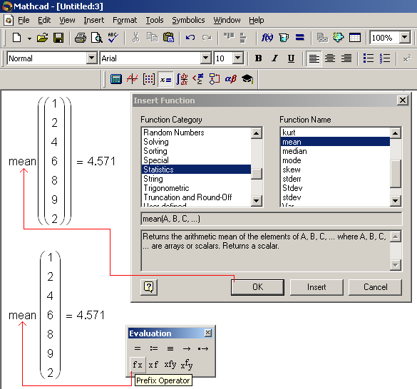
function mean
returns arithmetic mean of arrays (vector, matrix or range). The first call of
this function in Fig. 1.28 is made in common form: as a function. Through
it two parentheses are appeared (it is like saying salt is salty) that may
confuse a novice user. He will try to delete excess parentheses not
understanding why it is impossible to do. The way out is to call the “matrix”
function (the function whose argument is a matrix) not as a function but as
prefix operator, which allows operand without parentheses (see the second
operator in Fig. 1.28).
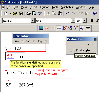
Figure 1.29
shows how to redefine built-in factorial operator to have it working with
fractional operands. For that we insert the function !(х) into worksheet being equal to built-in gamma
function which argument is shifted to one. We can call this new function in
traditional form !(5.01)= but to call as shown in Fig. 1.29 , as
postfix operator, is better.
Comment
How to insert the
symbol ! and other reserved characters into Mathcad
worksheet not in the form of operator (in this case, factorial sign) but as a
function name is described in sec. 1.2.2.
The
examples shown in Figures 1.28 and 1.29 are simple and have no practical value.
Still, using postfix and prefix operators to work with relative scales of temperatures
is very convenient. We will discuss it in sec. 1.4.
Fig. 1.30
shows how to insert additional Boolean operator “approximately equals” by means
of infix operator into a worksheet. It is very useful in performing iterations
(See ch. 6) where loops stop
execution by “approximately equals” instead of “not exactly equals to”. Fig.
1.30 shows that p
approximately equals to 3.142 but the value 3.14 (which we remember, as a rule)
is not “approximately equals” to p.
Fig. 1.31
shows that after we have redefined two-operand built-in operators addition and
multiplication the hierarchy of the expression 2 + 2·2 is opened (we discussed it above) by
means of the tree operator.
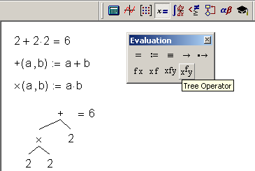
One of
the causes that Mathcad has become popular is that a user can insert as
operators, as functions into a worksheets depending which he may have got
accustomed to when learning mathematics in school or in institute. This makes
the Mathcad worksheet looks like a paper with calculations made by hand or in a
text processor environment (Scientific Word, ChiWriter etc).
Nevertheless,
our advantages in place can lead to disadvantages in other places. Live Mathcad
equations using many-storied operators, instead of text functions, cause
difficulties in Mathcad Application Server technology (See
1.2.2. Variable name
While the
names (symbols) of built-in variables, functions, and operators are fixed, we
may give any name to a user object. The limitations here are connected, first,
with certain traditions (discussed in sec. 1.3),
and secondly, with the features of Mathcad itself.
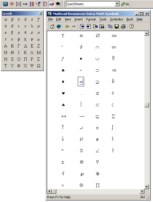
Fig. 1.32
shows symbols, Greek letters and special characters from the Mathcad Resources, which we may use in
addition to the keyboard characters to name variables, functions, and
operators.
Comment
The Greek toolbar
also contains two mathematical instruments — constant p and gamma function G.
Combination
keystroke <Shift>+<Ctrl>+<k> allows us to insert in variable
names first, the symbols prohibited from using in traditional programming
(blank, dash, comma, etc), and, secondly, symbols fixed for some operators in
Mathcad ($, @, etc). After pressing this
combination, the color of pointer changes from blue to red that indicates
emergency state of Mathcad. It prevent us from inserting certain operators by
fixed symbols, for example the assignment equal sigh by typing <:> (see sec. 1.1). The symbol just will be
added to the variable name which has been finished already as we type symbol
<:>. To change the pointer color back to blue we should type the symbols
<Shift>+<Ctrl>+<k> again. Fig. 1.32 shows that this
combination allows us to insert nonstandard but “speaker” variable names: US$, etc.
Only one
character, which we cannot insert into the variable name (or rather, we can
type but cannot see it then), is a period. It divides the name into two parts —
name itself and a subscript, for example, typing t.вх we obtain tвх. Nevertheless, we can do that
creating a variable with a text subscript, which has an invisible blank as a
name before subscript and periods as subscript. For example, in Fig. 1.4
two periods were inserted into unit of pressure мм рт.ст. and into unit of capacity л.с.(horse-power) in this way — see Mathcad
worksheet at http://twt.mpei.ac.ru/MAS/Worksheets/Book_MC_12/1_04_Insert_Unit.mcd.
A reader
can see a blank (space) in the beginning of the variable name мг-экв/л, shown in Fig. 1.33. This blank is not
fortuitous: some characters cannot stand in the beginning of variable names.
First of all, that concerns digits 0 through 9. If the variable name consist of
one character, which is a digit, that follows to such curious thing 3:=7
7:=3 —
the variable named 3 assigned the value equals to 7, and the variable 7 equals
to 3, etc. Sometimes (in certain Mathcad versions in combination with certain
Windows versions) some letters of Cyrillic alphabet cannot stand in the beginning
of a name. Although, that restriction does not apply to a blank. Therefore, it
is desirable to start a questionable name with a blank. A blatk or some of it
may use as a variable name making it invisible (see sec. 1.2.3).
Another
way to enter a sophisticated variable name into Mathcad worksheet is by
pressing <Shift>+<Ctrl>+<j> (Fig. 1.34).
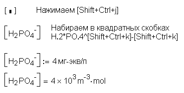
Fig. 1.34
shows how to enter the variable with rather a complicated name H2PO4-(one-valent ion of orthophosphoric
acid) that practically consist of three variables: the variable H2 (H.2) multiplied by variable H2 (H.2), which, in turn, raised to power minus –
(<Shift>+<Ctrl>+<k>+<->). There is a limitation: such
complicated names are enclosed in square brackets.
Mathcad 12
has the third key combination <Shift>+<Ctrl>+<n> that enters
a system index into the variable name. This index contains one of four key
words: mc, unit, user, and doc enclosed in square brackets.
Comment
System index is
the third type of that in the variables. The previous indexes are text (t.вх) and digital (V[i).
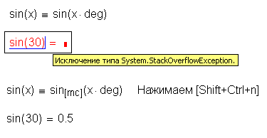
Fig. 1.35
shows defining (redefining) sin(x)≡sin[mc](x·deg)by the new system index. Mathcad
users sometimes need to have the function sine work with degrees but not with
radians. In this case, the native Mathcad function is used to omit memory
overflow through recursive function calls.
There is
one more reason to introduce the system index into Mathcad. As we noted before,
the worksheet may contain different variables of the same name. This is a
typical example beside of those shown above — the conventional mathematical
notation f:=f(x):
the variable f is
assigned the value of function f with the argument value saved as variable x. To avoid errors these two objects must be
divided by styles. Although, such Mathcad worksheet is impossible to enter “at
sight” in which we cannot see a style of a variable or a function. That is why
the notation f:=f[mc](x)is better. Although, that may be worse as the excess information makes a
worksheet hard to read and study.
Comment
Using styles is a
kind of coding, encipherment of a worksheet: everything is computed right but
is impossible to renew a worksheet.
As will
be discussed in sec. 1.5,
Mathcad worksheet is three-dimensional. That allows us to overlap the variable name
by a picture, its graphic pseudonym, and remove the restrictions on the
variable names, for example, insert a period of two indexes without across
shift (see Fig. 1.34). Fig. 1.36 shows the problem on population
growth of wolfs and hares; the pictures of the animals substitute the variable
names.
Fig 1.36 Fig 1.36a
Fig 1.36b
Fig 1.36c
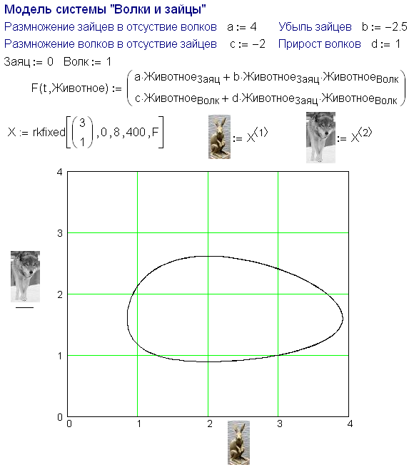
It is
impossible to use variable names with “pseudonyms” on Mathcad worksheets
assigned for further modifying. Those are appropriate in Mathcad worksheets
opened on the Web.
1.2.3. Invisible variable
This
section considers an unusual problem: is it possible and expedient to have
invisible symbols on the screen? The answer: it is possible and expedient.
Moreover, this technique does not hide something from a user but makes a
worksheet easier to read.
Everybody
knows the history of invisible man by Herbert Wells and numerous screenings.
Here is a story of invisible variable (constant, function, operator). Its life
is possible and in a number of cases is expedient not only in Mathcad and but
in other applications.
As was
noted above Mathcad allows us to change the color of the variable font. White
color is a mixture of seven rainbow colors in existence but a color equal in
rights and appropriate to paint variables in Mathcad. At that, if a white
variable is situated on a white background it becomes invisible.
A brief
mention about colors in Mathcad worksheets. By default Mathcad user type in
black-blue on white: mathematical expressions are black and comments are blue
(see sec. 1.3). Besides, by
default these two objects have different fonts: mathematical expressions have
it san-serif, text — ordinary that allows us to make them out in
black-and-white hard copies, for example in prints.
Comment
Default choices
for font and its color refers to a template, a empty worksheet that we see on
the screen when we first open Mathcad or click the button New on the Standard toolbar. The name of the
template is normal. When Mathcad executes command New from the File
menu it displays the dialog box containing the list of built-in and users
templates that differ from the standard (normal) in arrangement and filling. We
can create a user template (another name is “Blank Worksheet”) choosing command
Save As. The file has extension mct and contains in Templates folder.
The background
of Mathcad worksheet is white[18]
(we type in black-blue on white). A user may change it for green, for example.
Comment
It is believed
that green color is good for vision (green lamp shades, spectacles with green
glasses etc). The Herculean displays typing in green on black were widespread
ten or fifteen years ago.
Moreover,
a user may change the background color of some expressions to make them more
conspicuous for those who will study a worksheet. Otherwise, one may hide the distinct
expressions changing its background from white to black (the invisible
expressions: we write in black on black[19]).
As we noted before a Mathcad worksheet may
contain different objects of the same name through the different styles.
А:=3 А:=4 А:=A+A A=3 A=4 A=7
This example shows (also see Fig. 1.9) not
one but three variables А
which save their values equal to 3, 4, and 7. Our example is rather artificial,
but real Mathcad worksheets quite often contains two variables А one of which is a user (such variable name is
very popular) the second is built-in (А is a unit of current strength).
Comment
Mathcad is not
just a mathematical but mathematical and physical environment. It allows us to
assign the variables not abstract values (as in traditional programming) but
the value of the physical quantities (mass, time, length, energy).
To be
able applying both ampere and operator A:= we must assign these variables different
styles. To omit the confusions we may change some font characteristics of the
variable style: size or color. The color may be white as well. That is a n
invisible variable, the hero of our discussion. In the Herbert Wells’s novel,
the invisible man became visible when got dressed. We can make visible such
variable in whole Mathcad worksheet highlighting some operators or changing the
background color of the worksheet.
Let us
consider the examples that justify using invisible variables and show the
benefit of them.
Example 1. Invisible addition
Mathcad
allow us to change the multiplication sign. A user may select the one from the
following:
2×а 2·а 2 х a 2 а 2а
The
multiplication sign is invisible in last two examples that conform to the
tradition existing in mathematics do not place a sing between efficients, if
the first is a constant and the second is a variable.
Comment
For that
reason, a variable name cannot start with digits.
However,
blank space between the two values may mean as addition, as multiplication. For
example, 2 hours 30 minutes, 1 kilometer 200 metes etc. Here
the invisible addition sign stands between the same quantities (time and
length), and multiplication sign — between the constants and the units.
Fig. 1.37 shows how to solve it in Mathcad.
First two
operators in Fig. 1.37 insert the user function named + into a worksheet duplicating the
built-in addition operator. We cannot change the style, therefore the color, of
built-in addition operator (that is not advisable: we need the “visible”
addition), but to change a user function is allowable that was done with the
second operator. Mathcad allow us to call a function with two arguments as an
infix operator adding up invisibly five feet and twelve inches, “the size of an
averaged Englishman”[20].
Fig. 1.37 also shows how to change the name of variable style from User 1 to invisible and the color of the
variables to white (see New Style Name in dialog box Equation
Format).
Besides,
the built-in operator of invisible addition for a vulgar fraction is appeared
in Mathcad starting from version 2001(Fig. 1.38). We can use it pushing
the particular button on the toolbar Calculator before fraction
introducing. It is also possible to use the invisible addition in the result
inserted by the evaluation equal sign = between the integer part and the fraction
after the corresponding formatting (format Fraction,
also see Fig. 1.6).
Example 2. Zero dimension quantity
Sometimes
Mathcad is too pedantic in dimensional quantities. For example, one says that some
equipment is situated at a height of twenty meters and another at zero and not
specifies the units of that zero (meters, centimeters, feet, or inches etc).
Nevertheless, Mathcad always displays the units of the dimensional values even
when it is not necessary. In that case we can hide an excess unit converting it
to invisible.
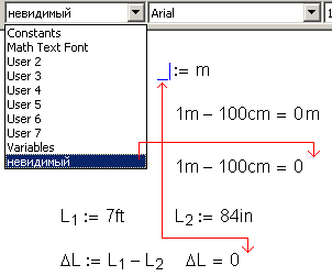
Besides,
the invisible unit appeared in Mathcad 12. Now the operator 1 m — 100 cm returns 0 but not
Example 3. The Roman
arithmetic
Mathcad
works with decimal, binary, hexadecimal, octal numbers. However, we may need to
make Mathcad work with forms more exotic, for example, with Roman numbers. For that
we insert the function with the invisible name that returns a Roman number if
its argument is an Arabic and conversely the Arabic number if the argument is
Roman (Fig. 1.40).
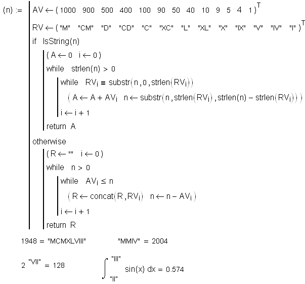
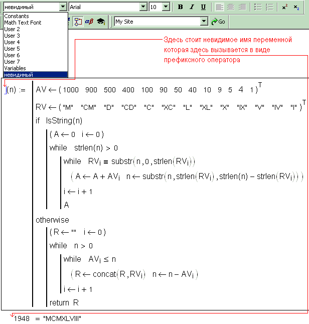
Fig. 1.40
shows the invisible function called as postfix or prefix operator which
arguments are not in brackets that gives the illusion of Roman arithmetic (see
also Fig. 1.28). Only quotation marks weigh down the Roman numbers.
Example 4. The dispersed
matrix
Mathcad
has powerful instruments to work with vectors and matrixes (arrays). There is
one limitation: these arrays should be completely filled. In practice we
sometimes meet with nonrectangular matrixes, for example, with triangular. The
matrixes may have more complicated form. Thus, in
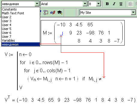
The empty
elements of the matrix in Fig. 1.41 keep the number that cannot be a
matrix element. We do not see it; it was assigned invisible style. Before
working with such matrix usually it is turned into a vector eliminating empty
elements by the small program that shows Fig. 1.41. Fig. 4.14 shows
more complicated program; it turns the matrix into three vectors.
Example
5. Displaying a dimensional value in several units
Often we
display the result of a computation in different units Р=760 mm Hg, Р=1 atm, Р=101.32 kPa etc. It is better to display here
only the first variable and put away the rest.
Comment
That is a good
general principle for all documents including Mathcad. If we can put something
away, we should do it.
Fig.1.42
shows the extension of the problem about capacity of the human heart which
displays the file Wсердца= = in two capacity units,
in watts and in horse-power.
Example
6. An endless loop
Mathcad
provides programming operators for creating for loops and while loops (See
We can
also insert other invisible symbols into the program, for example, to insert an
empty string or to shift an operator to the right for fixation of the cycle
nest.
Example
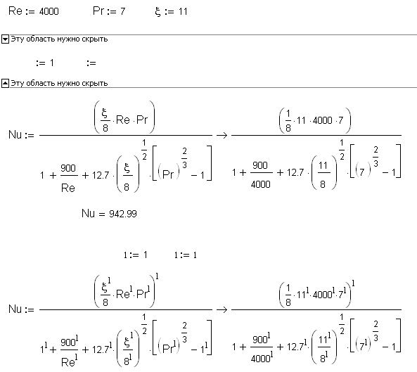
It is known that introducing a variable value
by the operator := we can display a numerical value by the operator ®.
This calculation technique was shown in Fig. 1.11. At that, if all the
variables of an expression have their numerical values operator ®
displays a result and not the expression. Still, (this is a Mathcad user’s
dream) it is desirable to see not only the resulting value of a variable (that
easy to do by the operator =) but the values of all variables forming the result (values of
variables Re, Pr, and x from the example in Fig. 1.44). Such displaying
is useful especially if the operators forming variable values Re, Pr, and x (speaking of
Fig. 1.44) are far from the operator forming the variable Nu that is of interest to us.
Fig 1.44
Fig 1.44a Fig 1.44b Fig 1.44c Fig 1.44d
We can display values of the variables Re, Pr, and x but we can also try to separate the resulting
numerical value into constituent values by two invisible operators and a ruse
that shown in Fig. 1.44. The point is that a variable l was inserted into the computation
(it is the narrowest) equals to 1. Then, all the variables in the tandem Nu:=...®... were raised to l degree but previously variable l is lost their numerical value for
symbolic conversions (operator l:=l). All the ruses result in that shown in Fig. 1.44.
Example 8. Comments in Mathcad worksheets
The previous Mathcad worksheets shown as
pictures are without any comments, texts or pictures that do not affect to
computation but help to understand its essence. Fig. 1.5 being an
exception shows Mathcad worksheet with fundamental physical constants as an
assignment operator (for example, с:=299792458·m/sec) and with text comments to the left
Velocity
of light in vacuum.
Besides, in the left top corner of Fig. 1.5 there is a name of the
worksheet and small graphic “adornment”.
Many users of Mathcad do not insert the
comments to the worksheets thinking that they are created for personal use and
elucidative fragments could be inserted later. Often this “later” never occurs:
all “non-comments”(mathematical operators) are inserted into the worksheet, it
works and gives precise result; there is no time to insert comments, we should
go further to develop this worksheet or to create the new one. Still, if the
worksheet is intended for personal use some comments in it will not be
superfluous. We may tangle even in own worksheet opening it after a time if it
have no any comment, for example a name.
Comment
We can name the
operator non-comment if the computation interrupts and displays an error
message when it being withdrew from the worksheet.
Returning
to the point of sec. 1.2 we can
contend that the best comments are right, “indicating” names of variables and
functions were fixed long ago on the definite quantity in a definite branch of
science. It will be enough to name such a worksheet and that will be clear
without comments.
Comment
A name and other
data concerning a worksheet (the time of creation etc) can be placed in the
heading and the “basement” of a worksheet by the command Header and Footer… from the View
menu. Mathcad 12 provides advanced features to save metadata (information
about information).
We can
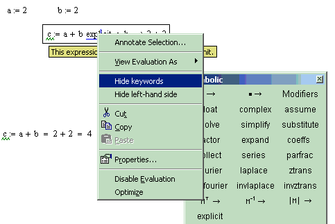
transform the pure mathematical operators to the comments clicking on it with
the right mouse button and selecting Enable/Disable Calculation
from pop-up menu (Fig. 1.45).
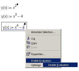
The
indicator that a mathematical operator is turned off the computation is a black
rectangle upward and to the right of it. We can disable operators to transform
it to a comment and, for example, to select the formulas for calculation from
the list available or to speed up computation. For example, a three-dimensional
plot can be disabled in checkout and be enabled again in ready worksheet. If
one function is defined twice its first definition can be considered the
comment under the certain conditions. There are Mathcad worksheets containing
whole pages that are the comments as a matter of fact. The developer of such
worksheet suggests users to study the calculation, after that insert their
data, and make computation. In principle, here the operator ![]() ≡
≡ ![]() should work which definitions
applies above it (global definition) but it inaccessible in Controls (see
Fig. 1.13) and in Web Controls (see Fig. 1.14) being used more
often to design an interface. Therefore, we ought to type again (duplicate)
calculation operators after inserting the source data and hide this area as
shown in Fig. 1.22, for example. Another way to transform the assignment
operator to comment is to substitute = for := (Boolean equals, but not the equal sign for
evaluation): c=a+b2 for с:=a+b2.
should work which definitions
applies above it (global definition) but it inaccessible in Controls (see
Fig. 1.13) and in Web Controls (see Fig. 1.14) being used more
often to design an interface. Therefore, we ought to type again (duplicate)
calculation operators after inserting the source data and hide this area as
shown in Fig. 1.22, for example. Another way to transform the assignment
operator to comment is to substitute = for := (Boolean equals, but not the equal sign for
evaluation): c=a+b2 for с:=a+b2.
This is a
general way to insert the comments. We type several symbols that is a name of a
variable or a function by default but it transformed into a text after pressing
a blank Thus the fact is marked that blanks can be in comments only but not in
the names of variables or functions.
Comment
Pushing the button
<"> (quotation marks) before inserting a comment or choosing Text from Insert menu we create a text right away. If the new comment is
practically similar to a previous, we should copy the old one and edit it.
We know
from sec. 1.2 that the names of
variables can contain blanks and other reserved characters inserted by
keystroke <Shift>+<Ctrl>+<K>. In this case, we can include
any symbol allowed in comments except for the period, which is known to turn to
invisible and indicate the beginning of literal subscript.
On the
one hand, the comment consisting on variable names is a typical mistake of a
novice user who does not know how to insert it right[21].
Still, there is another extreme of this phenomenon (the comment consisting from
variable names).The most experienced users make all the comments or part of
them as names of variables preparing their worksheets to publication in Web
(See
The
pictures are very informative in Mathcad worksheets. We create a picture
elucidating the calculation in graphic applications (in Paint included into
Windows) or scan it from a book and insert it as part of one object of Windows
application to another.
Comment
Often Mathcad
includes the SmartSketch application that works with vector graphics but not
with bitmapped one. In addition, Mathcad can exchange data with applications
such as AutoCAD.
If we
double-click this picture in Mathcad, causing in-place activation of the
originating application we can edit it, for example, in Paint and return to
Mathcad (Fig. 1.46).
We can
insert parts of Mathcad worksheet itself into the picture “freezing” (button
<PrintScreen>) it and transferring the “freezing” to graphic application.
For example, by this way we can transfer names of some variables from Mathcad
worksheet without changing their fonts and other attributes.
We can
insert the picture both manually and automatically selecting Picture from Matrix toolbar — see Fig. 1.47.
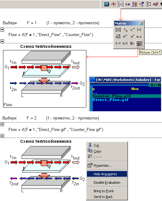
Fig. 1.47 shows the Mathcad worksheet where
variable F is assigned the value 1 or 2 (not 1) which change
the value of variable Flow from Direct_Flow to Counter_Flow following
the scheme displaying of cocurrent or counterflow
heat exchange. These two pictures made in advance in the graphic application
(Paint) were saved as Direct_Flow.gif and Counter_Flow.gif. Fig 1.47 shows
“edge” of screen displaying two image files in File Manager “FAR” (the analogue
of Norton Commander).
To change
the pictures in Mathcad worksheet according to the way of calculation is a very
useful technique (one may say change of decor). That allows us, for example, to
change from Russian into English, modify a set of visible formulas of
calculation, etc (See
“Change
of decor” may imply change of the languages. Thus, Fig. 1.48 shows the
content of the hidden operators that display the correspondent text according
to the chosen language (choose defined switch). The texts are saved as separate
image files. See the Internet version of the file at http://twt.mpei.ac.ru/MAS/Worksheets/Therm/V_balloon_add_ER.mcd.
Fig. 1.48 shows part of a screen with Explorer containing these
four image files.
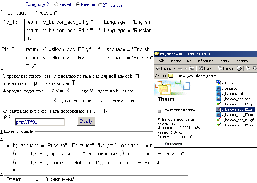
Although
we will return to texts that are the lion's share of comments.
Mathcad
has the spell-checking but for English texts only.
For that
reason to create texts in Mathcad, it is better to type that in Word or insert
Word itself into Mathcad worksheet as shown in Fig. 1.49.
By the
way, finally Mathcad 12 allows us to choose language in menu commands,
references and other comment environments of this mathematical program
Fig. 1.49
also shows new Language tab
available in Mathcad 12. We can change not only spell check language via
it (clicking Spell Check Options) but language in menus and dialog boxes
(top scrolling list Menus and dialogs) and also some mathematical
expressions (top scrolling list Math language). Earlier versions
(Mathcad 8-11) have only British and American dialects in spell checking.
Mathcad 12
enables us to comment separate operators via View | Edit Annotation... from pop-up menu clicking on it with the
right mouse button (Fig. 1.50).
The
operator having such a comment is distinguished by additional brackets appeared
when we move a pointer to it. Besides, we can recall Excel allowing us to
comment the table cell. The sign of a comment is a corner in the left top of a
cell.
We can
attach more sophisticated “comment” information in Mathcad 12 via command Properties
from File menu (Fig. 1.51).
Such
information about the file (metadata) can be necessary to distribute in Internet
with technology Mathcad Application Server (See
1.4. Calculation
with physical quantities: problems and solutions
In the
beginning of this chapter, we noted that Mathcad is not just mathematical
application but physical and mathematical (see Fig. 1.4 and 1.5).
Frequently, the real “physical” calculation, i.e. that where almost all values
have units (mass, length, force, etc.), have units not as a multiplier, simplifying
and allowing us to avoid some errors, but as a comment of the kind: enter pressure
value in atm Р:=120 instead of more convenient enter pressure
value Р:=120 atm.
Comment
Chapter 7
tells how to simplify and automatize the unit choice from the offered list by
interface elements Controls and Web Controls changing the operators of the
type variable = quantity·unit to more convenient.
What are
the reasons of imperfect using the Mathcad capabilities? The first one is, of
course, that some users do not know about such useful Mathcad tool as built-in
constants of physical quantities and use techniques in Mathcad, in physical and
mathematical program, formed by “non-physical” languages or by electronic
worksheets where the variables keep only numerical values and units are noted
in comments even not always.
The
second group of Mathcad users does not use units explaining that their
quantities expressed in the basic units of one unit system (for example, in SI)
and they have no difficulties with unit conversion. This reason is fortified
with that without units Mathcad worksheet is simpler to compile to environment
of the programming languages, for conversion of customized functions into
built-in in the form of DLL. The third reason is major. It is connected with
some peculiarities and limitations of unit tool that cause a skilled user to
seize units from a worksheet, almost finished, and turn them into comments:
instead of
Enter pressure value Р:=120 atm
there is
enter pressure value in atm Р:=120
Physical values
in a calculation can be considered as appropriate comments in a Mathcad
worksheet (see sec. 1.3) without
going into their “physical” root. The operator P:=120 is silent but that Р:=120 atm does not require additional
comments. One more feature, connected, if it is possible to say, with
“psychology” of Mathcad worksheet creating, brings together units and comments
– they retard writing, draw away the core. Unit insertion is often postponed
for future just as comments. Afterward, calculation gives acceptable result...
The tool
of units in Mathcad is rather simple. We just type a variable consisting of a
number followed by a unit name, user or built-in. We type the unit or insert it
from Insert Unit dialog box shown in Fig. 1.52.
Comment
If we type the
unit name, Mathcad writes multiplication sigh, visible or invisible, between
value and unit. The form of this sign (point, cross) can be changed.
Fig 1.52 Fig 1.52a
Fig 1.52b Fig 1.52c
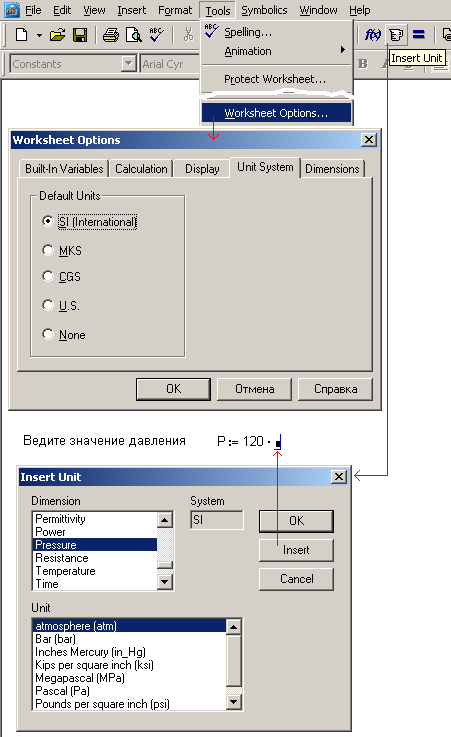
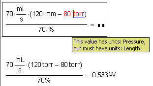
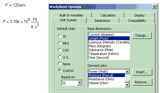
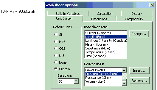
Fig. 1.52
shows Unit System tab from Worksheet Options dialog
box with SI unit system set by default. Mathcad checks calculations for
dimensional consistency: we cannot add meters and kilograms. That allows us to
avoid errors and misprints in formulas, for example, wrong power or addition
sign instead of multiplication.
Comment
Dimensional
checking is disabled in plotting (see sec. 1.6).
Displaying
dimensional value by operator ![]() =
= ![]()
![]() we can insert another unit into the
third operand (into the third rectangle appeared when we hold the pointer over
operator) to obtain required result or, rather, to change a unit by default to
another. We can also duplicate dimensional value with different units to give a
choice for a reader: joule and calorie, atmosphere and megapascal, etc (for
example, capacity of human heard expressed in watt and in horse-power).
we can insert another unit into the
third operand (into the third rectangle appeared when we hold the pointer over
operator) to obtain required result or, rather, to change a unit by default to
another. We can also duplicate dimensional value with different units to give a
choice for a reader: joule and calorie, atmosphere and megapascal, etc (for
example, capacity of human heard expressed in watt and in horse-power).
What cause
the skilled users to keep of units or seize that from almost finished
worksheets?
There are
some pitfalls:
1.
Some
Mathcad tools are not adapt for working with dimensional values. They are
interrupted with the error message “Can’t have anything with units and
dimensions here” (finance functions or functions working with splines) or
return wrong answer (function line). In that case, we should take off the dimension dividing the variables
to correspondent basic units and then return required units multiplying it by
the value. Such examples (temporary, not complete disabling unit tool) you can
find in
If the work with dimensional values is not
planned, unit tool should be enabled via command Tools | Worksheet
Options... and switch None in Unit System tab.
Otherwise, unit tool may result in errors. For example, a user forgot to define
a variable that has the similar name with a unit; nevertheless, the calculation
is not interrupted. Here is incomplete list of such “crafty” variables: A, K, T, S, R, m, L, s, etc.
Another example. A user defines a function and wants to represent it as
QuickPlot, i.e. without defining a range variable previously, for example m:=–3, –2.9.. 5. In result, a plot is not displayed or, rather
only one invisible point is represented because variable m keeps the length unit – meter.
2.
Mathcad
symbol mathematics work with units as with variables neglecting that one meter
amounts hundred centimeters or sixty minutes are in a hour, etc. Symbol
mathematics is foreign element in Mathcad; it was taken from Maple where unit
appeared in the eighth version. Although, symbol mathematics is auxiliary tool
in Mathcad integrated seldom into a calculation but operates auxiliary
functions. If it is necessary to have units worked in symbol mathematics we
should make efforts: enter to Mathcad via operator substitute that 1 m=100 cm, 1 hr=60 min, etc.
3.
Mathcad
arrays contain only dimensionless quantities or the quantities having the same
unit, i.e. the same quantities, time, force, mass, etc. Only one exception from
this rule is known. Function Find returns a vector of values with different
units if its arguments have different units. If it is necessary the function
created by program to return several values with different units in one vector
or matrix we may take them off and later return them back (for details see Ch. 5).
4.
Sometimes
we have to use so-called empirical formulas[22]
connecting not just quantities but quantities in the appointed units. In that
case we should also take steps similar to that described in point 1 to
avoid fails in unit use. As example, Fig. 1.53 shows the calculation of a
secondhand car cost depending on its age and run.
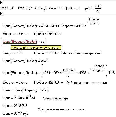
The way in which the formula of car cost was
obtained is discussed in
Introducing the empirical formulas, we always
clearly define the units for source data and dimension of the result. In that
case, car age should be expressed in years and run –in miles. The formula
returns cost in US dollars[23]. These units should be added to the formula and we must disable unit
tool temporary (see point 1) in it. We did it when we redefine the
function Цена(Возраст, Пробег):=...dividing the arguments to their units and
the function itself was multiplied by required unit as shown in Fig. 1.53.
5.
Mathcad
list of units includes not all physical and other quantities that we have to
deal with. For example, there is no units of information (bit, byte), units of
cost (dollar, ruble, euro, etc) can be necessary on calculations. Mathcad works
only with “The magnificent seven” of SI (length, time, mass, current,
temperature, illuminosity, and substance) and with their combinations (force,
power, energy, etc). What we have can do in Mathcad to make technological and
economic calculations dealing with dollar, ruble, euro, etc? Fig. 1.53
shows one of techniques. Dollar ($US) is assigned a unit which is not used in this calculation, and
generally rarely used in calculations, for example, candela[24]
$US:=сd. Then we can attach other currencies to
dollar, for example руб:=$US/29.After that the cost will be
displayed in candela (see Fig. 1.53) which we should replace with the
required unit (pseudo-unit) of the cost.
6.
We
sometimes meet formulas purely physical in essence and empiric in their form
(see point 5). Fig. 1.54 shows the example of working out such
formula in the following problem: it is given an efficiency of a power station
(h) and we shall find consumption of equivalent
fuel (bут) for power output. All courses give
the formula for such calculation: bут=12300/h where (h) should be expressed in percents
and result (bут) will be in grammes per
kilowatt-hour. An example: 12300/32=384.4 —power station having efficiency 32%
burns
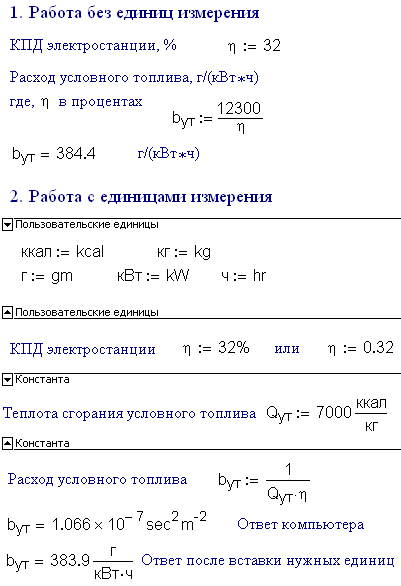
If the appropriate units are listed in the
comments, we can have this formula works correctly by the method described in
point 4. Although there is another way -- such pseudo empiric formulas
were derived to free us from additional calculations connected with units. At
that, if the coefficients obtained are easy to memorize, as in our case – one,
two, three, and two zeros, such simplified formula settles down in the courses.
Source formula for calculation of equivalent fuel consumption is: bут=1/(h·Qут), where Qут is heat of combustion of equivalent
fuel, the accepted value of it amounts 7000 kkal/kg (easy to remember
too). If we insert this formula, but not simplified, work of Mathcad unit tool
will not be disturbed (see Fig. 1.54 at the bottom).
7.
Mathcad
uses only absolute scale for units.
Particularly, that means if the quantity equals to zero we need not to assign a
unit. Nevertheless, we should do it in Mathcad, for example, l:=0 m, for proper work of dimensional
checking[25]. Although, there are relative scales too. For example, we
measure temperature in centigrade degrees (relative scale) but not in Kelvin
(absolute scale). Particulary, that mean the expression t:=25 °C contains not the multiplication sign between numerical constant 25 and unit °C but something else masked by blank.
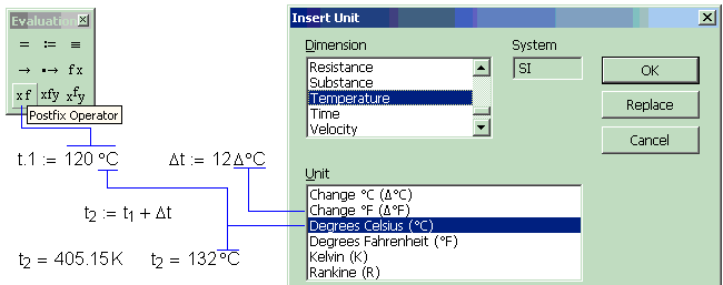
Fig. 1.55
shows one of solutions of relative scales basing on a simple problem. It is
given the input temperature t1 of a certain heater and difference of
temperatures in input and output Δt. We should find the output temperature t2. The problem is clear to be not
arithmetical but metrological. To solve it we insert three objects named C: the function named C and two constants of the same name,
the first (°C:=1) has style (°C:=1), the second (°C:=K) has style (°C:=K) and also we insert function with
invisible name (t):=(T/K-273.15) (see sec. 1.2.3).
Comment
There is not “degree”
sign in the keyboard. It is inserted by keystroke <Alt>+0176 or by coping
from Mathcad set of mathematical symbols.
All
objects are of the same name C but they are different having different styles (see sec. 1.2).
Working
with temperature expressed on the relative scale three situations occur. The
functions and constants described above help to solve these problems.
r
Situation 1. We need to insert temperature value
in centigrade degrees. For that, function °C with style Variables is called
(the first object named °C) as the postfix operator in the
right part of assignment operator := -- t1:=120 °C. At that, we assign temperature
value on the absolute scale to the variable t1.
r
Situation 2. We need to insert temperature
difference. Here we can use common Mathcad rule and multiply the value by the
unit K or °C equal to K (the second object named °C).
r
Situation 3. We need to display temperature value
in centigrade degrees. For that, we should turn the variable into operand of
the prefix operator with invisible name in the left part of operator :=. At
that, if we multiply displayed value by the constant °C equal to 1 (the third object named °C) we will get illusion that
temperature is represented on relative scale t2=132 °C.
Three
techniques and three objects of the same name described above allow us to work
with temperatures: insert temperature value on any scale, display temperature
value, insert and display temperature difference. At that we should apply
simple but important rule: inserting and displaying temperatures in any scales
use only absolute scale, Kelvin, in computing. Mathcad worksheet with
temperature conversion on different scales is accessible at http://twt.mpei.ac.ru/mas/worksheets/Temperature_Recalc.mcd.
There is
another unit that may cause difficulties in Mathcad – decibel (dB). Bel is the
decimal logarithm of the ratio of two quantities with the same units[26]
and decibel is correspondently a one tenth of bel. Measuring something in
decibels[27] we create a scale
(logarithmic) of the quantity values. At that, we should choose the base from
which begin calculations. In Fig. 1.56 we created such scale for capacity.
The base was accepted capacity of human heard (see Fig. 1.4)
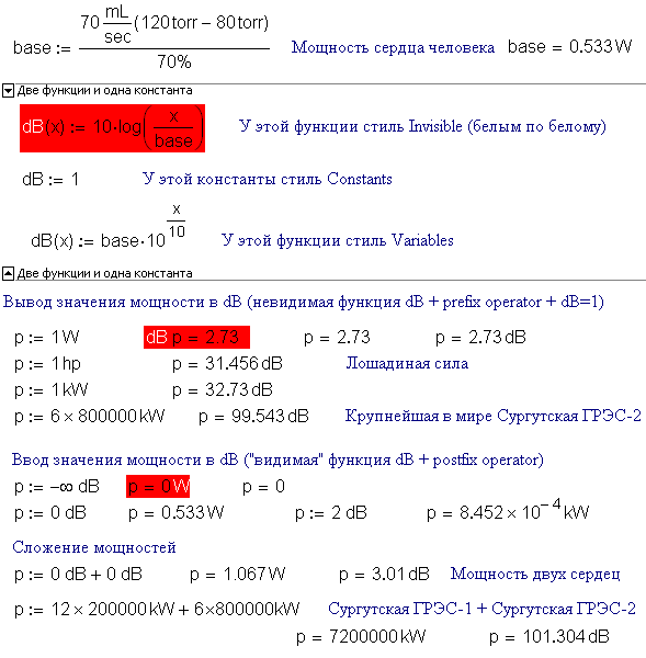
Two
functions and one constant are introduced in Mathcad to work with decibels.
Their names are the same, dB; name of one function is invisible written in
white on white[28]. These objects are different
because their styles are different. The invisible function is used to display
the value in decibels and that visible to insert. As with temperature, it is
called as postfix operator: not p:=dB(0) but p:=0 dB that imitates dimension.
Working
decibels (bels, nepers) the base (source value) is indicated sometimes too;
thus, p:=100 dB (re 0.533 W) where re is the initial letters of reference. Such way of working with decibels requires
not prefix but infix operator shown in Fig. 1.57.
Comment
This technique
does not work in Mathcad 12 because some changes were made in the on error operator.
Fig 1.57
Fig 1.57a Fig 1.57b Fig 1.57ba Fig 1.57c Fig 1.57d
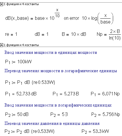
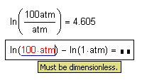
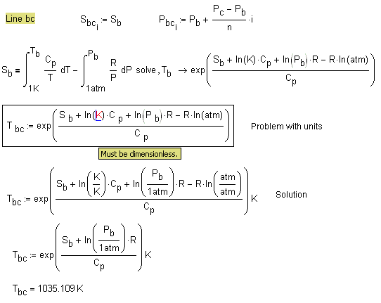
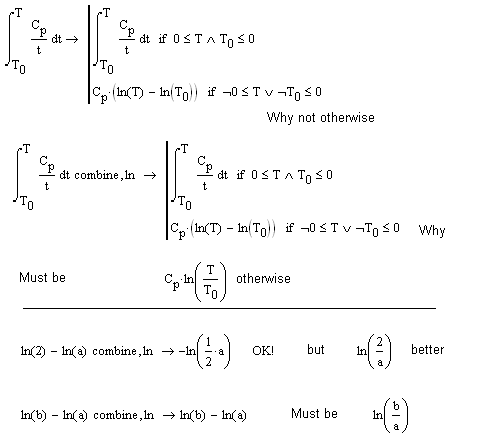
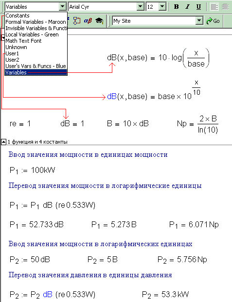
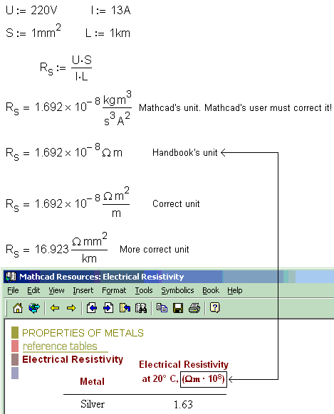
We can note some difficulties in using so-called
dimensionless physical values: plane and solid angles, mass, mole, and
inclusion volume fractions, etc. These problems occur in Mathcad too: in
version 12 steradian has become dimensionless (sr=1), earlier it had dimension (sr=1 sr). On the one hand, the developers restore logic by that: radian (the
ratio of two lengths) was dimensionless earlier while steradian (the ration of
two areas) had the dimension. On the other hand, that clears the way for some
errors of the kind: radians and steradians addition, sine of steradian, etc.
We can face with the problem of lack of dimension
checking working with other “dimensionless” quantities that have different
dimensions. While we cannot add mass and moles, addition of mole and mass
fractions will not result in a error message.
The dimensionless value, item, is often met in
calculations. As a rule, it is inserted into the worksheet as it=1 and then
work with it in the known way: Number of tubes in heat exchanger N:=2200 it, for
example. At that, the variable N remains dimensionless. Although, we can
remind that Mathcad keeps built-in unit for items (base units) – that is mole.
Mole divided by Avogadro constant is item which could be used in calculations.
Fig. 1.58 shows finding velocity of water in a certain heat exchanger; the
tubes number (nтр), interior diameter (dтр), and volume consumption of water (Q) are known.
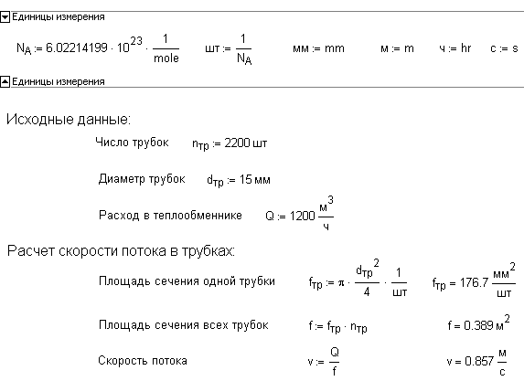
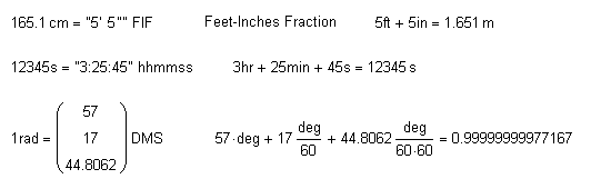
Dimensional items and other quantities with
“dimensionless units” seem to be just curious things. Thus, in a calculation
shown in Fig. 1.58 cross-section area of one tube and total area of all
tubes have, strange as it may seem, different dimensions: mm2/it and
mm2and they cannot be added. That is right – such operation can be
done only by mistake. The example shown in Fig. 1.58 is strained, of
course. Nevertheless, the author knows real example when the mistake in
sophisticated technical and economical calculation was found only after the
heading operators руб:=cd and шт:=mole were
substituted for руб:=1 and шт:=1. It turn
out, that in wrong calculation two quantities were added with dimensions руб and шт.
We sometimes ought to have two variables with
different dimensions for one quantity. That is, for example, the temperature in
thermodynamic calculations where variable t assigns centigrade
degrees and T – Kelvin. Mathcad unit tool allow us to avoid this
bisection.
When the author sees a student’s calculation of a
“physical” problem made in Mathcad without units it resembles to him situation
when one makes calculations in Word: types formulas there and calculates
manually, on Windows calculator (see Fig. 1.2) or often on the single one
lying not far from computer keyboard.
On the other hand, a reader can see in Ch. 5
two particularly “physical” problems with meters, kilograms, seconds
(Fig. 5.14 and 5.16); one of which has no units (Fig. 5.14) and
another contains units only to display results (Fig. 5.16) because the
main function of these calculation odesolve does not work with
dimension arguments. That occurs in Maple too that can work with units to
starting from version seven but its feature is not global. Therefore, the
programs and users should meet half-way to return completely dimensions into
the calculations.
1.5. Three
dimensions of Mathcad worksheets
As was
noted in sec. 1.1 Mathcad has one
special feature standing out from other applications. Mathcad worksheets are
“three-dimensional”: beside the coordinate axes above/below (let us call it
x-axis) and right/left (y-axis) there is the third one: close/farther (z-axis).
In Mathcad, it is possible to overlap two objects and select which will be in
front of another. Fig. 1.59 shows the situation where the texts Гипербола and Парабола are overlapped the plot and
indicate correspondent lines.
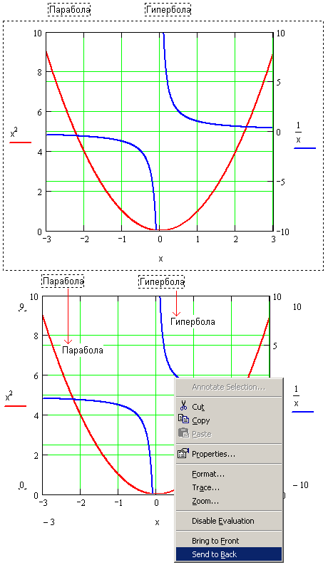
The features indicating the third dimension of
Mathcad worksheet are two additional commands, Bring to Front and Send
to Back, from pop-up menu.
Choosing a command from the menu, we can move an object.
Appeared in version 2000 of Mathcad the third
dimension became widely used right away.
Comment
Mathcad adopted
this feature from Word and Excel that enable objects overlapping too.
The
example shown in Fig. 1.59 (inscriptions on the plots) is the most
widespread.
Comment
The inscriptions
on the plots can be made transparent if needed, not in Mathcad but in Paint,
for example, if we insert it there to redesign (see sec. 1.6).
Here are
two examples less known to Mathcad users. Fig. 1.60 shows Mathcad function
created by a program Min_GR that returns coordinate of the point x, the minimum of another (analyzed) function
dividing the segment in golden ratio.
It is
known that Mathcad programming tool have no instruments to make comments in
programs and it did not enable us to have a local function there until version
twelve. Nevertheless, Fig. 1.60 shows us comments: texts with different
fonts, Mathcad operators (a/b=b/(a+b)), and also a picture that is an exotic object
for comments in program. Besides, the program contains subroutine Golden_Ratio that has all features of a local
function although the worksheet was created in Mathcad 11 in which the
local functions are impossible. What is the matter? The matter is that all
these objects (texts, pictures, operators and even working function Golden_Ratio ) were placed on function Min_GR that gives an illusion of a single
well commented program.
Comment
To make the
function Golden_Ratio visible within function Min_GR we should use operator ≡ but not := which sigh is replaced by =.
The third
dimension can be used to hide some information in Mathcad worksheet. There is a
well-known literature rule, and the author[29]
of this book tries to follow it, to omit a word, a sentence, a paragraph, a
chapter if it is possible to do. In informational technologies this principle
(its motto is known:”Brevity is the soul of wit”) results in demand to omit
unnecessary, overhead information that prevent to read and understand the
electronic document probably more than absence of the comments. Such
unnecessary information is hidden in close areas of the Mathcad worksheets or moved
over the right border of a screen. If it is impossible to do, we can overlap
this information by additional or neutral comment as shown in Fig. 1.61.
Fig. 1.61
shows the problem, from safety engineering at power stations, coming to the
equation solved symbolically by Mathcad operator ![]() solve,
solve, ![]() ®. This operator “shoots” both to the left
(assigns the result to variable t ) and to the right (displays answer, turned out to be unnecessary,
which is overlapped in Fig. 1.61 by the comment)
®. This operator “shoots” both to the left
(assigns the result to variable t ) and to the right (displays answer, turned out to be unnecessary,
which is overlapped in Fig. 1.61 by the comment)
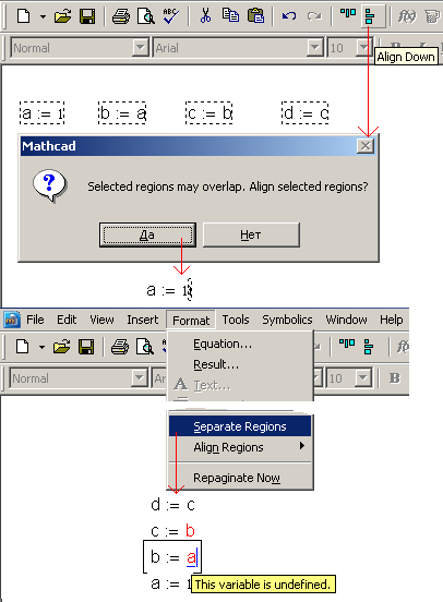
Fig. 1.62
shows the way in which four operators alighted horizontally can be realighted
in z-direction, axis perpendicular the display plane.
1.6.
Mathcad plots
One of
the most effective methods to represent source, temporary, and obtained data is
plotting. To continue comparing Excel and Mathcad started in this chapter, we
may say that the first application possesses business plotting and the second –
that scientific.
In
Mathcad, we can create plot via command Graph from Insert menu or
via the toolbar of the same name shown in Fig. 1.63. Mathcad plots are
divided rather relative on following groups:
r
The
plots displaying dependences (functions and arrays) of one variable: X-Y Plot,
Polar Plot, and 3D Scatter Plot;
r
The
plots displaying dependences (functions and arrays) of two variables: Surface
Plot, Counter Plot, 3D Bar Plot, 3D Scatter Plot, and Vector Field Plot;
r
flat
plots (2D): Х-Y Plot, Polar Plot, Counter Plot, and Vector Field Plot;
r
Three-dimensional
plots (3D): Surface Plot, 3D Bar Plot, and 3D Scatter Plot.
It is the
author’s opinion that such classification is better then given in documentation
and references:
r
2-D
plots: X-Y Plot, Polar Plot;
r
3-D
plots: Surface Plot, 3D Bar Plot, 3D Scatter Plot, Counter Plot, and Vector
Field Plot.
There are
more plot types then noted above where we listed practically the buttons on the
plotting toolbar (see Fig. 1.63) rather than types of plots. Some plots,
which could be considered as independent group(2-D Bar plot of graph of
errors), are displayed by correspondent formatting of the others, X-Y Plot.
We should
note that 3-D plots are rather promotional thing than a method to represent
results of large calculations, having practical aims not presentation or
advertising, especially, if we should print such plot where we cannot rotate it
to see from another point.
Comment
We can
rotate 3-D plots by specifying coordinates, changing values of three numbers in
the dialog box or with the mouse. If the mouse has a center wheel we can rotate
the wheel to zoom in or out of a three-dimensional plot.
Therefore,
considering screen and paper of printer to be flat, we should prefer simple 2-D
dimensional plots creating Mathcad worksheets. Real sophisticated problems may
base on set of functions with three, four, and five arguments which plots we
must represent correspondently in three-, four-, and five-dimensional space. We
should remember that complicated plots often hide rather trivial calculation
that masks itself with perspective, lightning, fog and other options. Complicated
calculation, having practical value, as a rule, is illustrated with simple,
plane plots, which represent the basic law of calculation. Such calculations
include set of curves, for example, instead of surfaces looking agreeably but
hard in work.
The most
commonly used plot on Mathcad worksheets is X-Y Plot. It represents
location of a couple of elements (components) of two, three and more vectors in
the plane, tabulation of functional dependences of one argument. Fig. 1.63
shows that two vector of equal size, x and y, were inserted, then a pointer was moved to
blank space where the graph to be appears, the button X-Y Plot was
pushed (or <Shift>+<2>, or <@> was typed). Variables x and y were placed in the appeared blank X-Y Plot (we can also insert there vectors
themselves). After that simple manipulations (vectors x and y also can be read from the disk or obtained in a calculation, not just
inserted manually) Mathcad represent a plot having a set of defaults. In
particular, the points of the plot representing the location of the couple of
vector elements are connected with a broken line starting from the first point
(the first elements of vectors) to the last one (the last elements of vectors).
We can change the default settings via the dialog box Formatting Currently
Selected X-Y Plot. It is called, as the other dialog boxes for formatting
Mathcad objects, with mouse double-click the graph.
Fig 1.63
Fig 1.63a Fig 1.63b Fig 1.63c Fig 1.63d Fig 1.63e Fig 1.63f Fig 1.63g Fig 1.63h
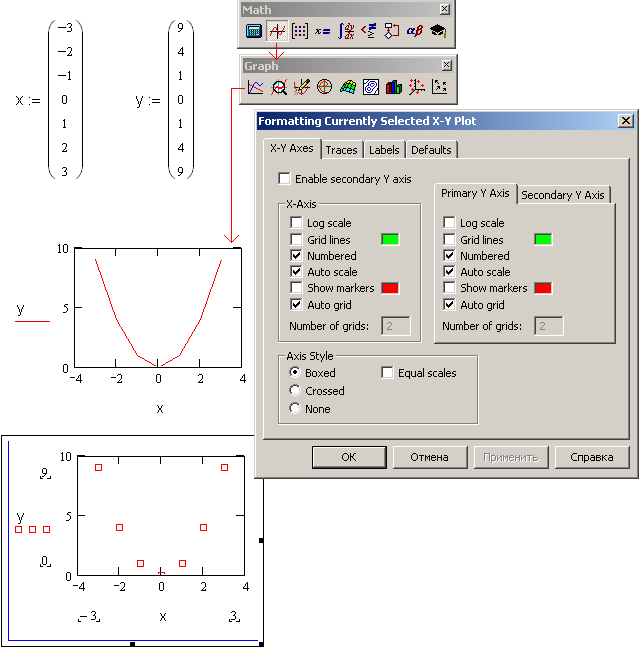
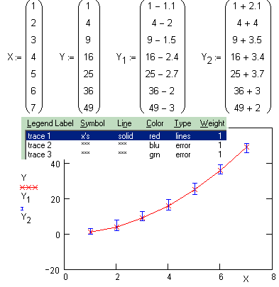
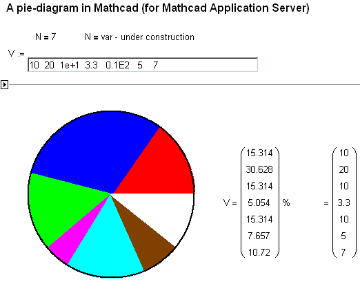
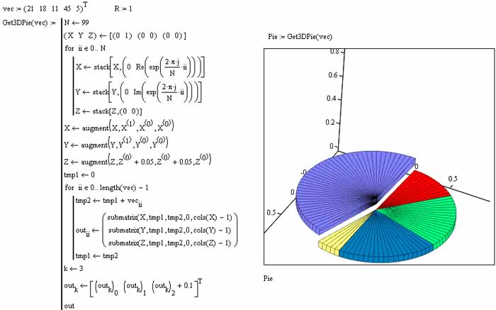
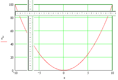
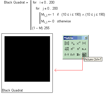
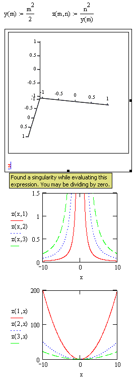
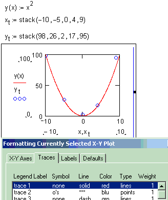
The plot
shown in Fig. 1.63 was reformatted in the following way: the lines were
put away (the word “lines” from the column Type was replaced for
“points”) and the boxes were substituted for periods, almost invisible, “none”
from the column Symbol. We should not, and it is needless to list in the
book all accessible changes in plots. That is desdribed in details in a user’s
guide and Mathcad references. We shall note only new features that appeared in
version twelve:
r
two
y-axes in a Cartesian plot (see Fig. 1.66 and 1.67)
r
change
of the marker color, four dotted lines (two horizontal and two vertical) by
which we can indicate special points in a plot, minimums, maximums etc.
r
adding
legends in plots, in one of four spare corners of a plot (and not just below as
in earlier versions) that makes a plot more compact.
Cartesian plots can
represent both couple of vectors and functional dependence themselves. For
that, it is enough to press X-Y Plot and fill in the placeholders of a
blank X-Y plot with the function defined above y(x) and its argument х, as shown in Fig. 1.63 but not
the names of vectors. After moving a pointer the plot will be produced over a
domain from -10 to 10 if the correspondent function returns real numbers in
this range. For example, square root of x will be represented within the range
from 0 to 10 because it returns imaginary numbers in the left part of x-axis.
At that, the problem comes to plotting of two vectors again: Mathcad divides
the segment of plot to points, the number of which depends on plot size on the
screen (on average it is 50) and on monitor definition, and computes the values
of an argument and a function in these points, i.e. forms two vectors to plot
them.
Comment
A user can resize
a plot holding the mouse button down and dragging the mouse.
Up to
version
The example in the
bottom of Fig. 1.64 shown displayed values of the variable х1 and function y1(x1) indicates that Mathcad draws plots point
by point but not as we studied in schools and institutes: first, find the
critical points (zeros, maximums, minimums, points of inflection) and then draw
a qualitative plot. We should remember about it creating plots in Mathcad. The
surfaces discussed below are created via the tabulation of a function of two
variables now. Then the correspondent grid of a matrix are risen at height
proportional to the values of function f(x,y) in the point (Fig. 1.65).
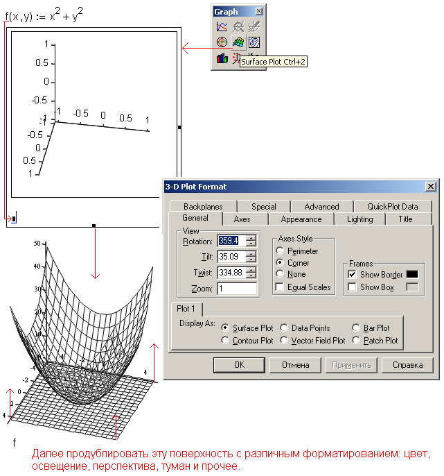
After
that, Mathcad formats this node in the following way: fills its cells with the
different colors over the various schemes, removes the grid, etc.
Comment
Number of defaults
of 3D plots (additional tools of formatting) is a dozen higher than that of 2D
plots.
Fig. 1.66
and 1.67 show the “graph” novelty of Mathcad 12: the second axis y of
2D plot in the example of finding the volume (V) and square of the liquid surface (S) contacting with air in the tank,
contained from a cylinder and two half-spheres, by maximum depth of a liquid (h).
The
second axis y allows us to estimate the volume of the rest of a liquid
both in м3 (the left axis) and in barrels (the
right axis). Then the question arises concerning the second x-axis to represent the height of the
liquid layer h (the
argument of function V) in an alternative unit, not in meters (the first x-axis) but in feet, for example.
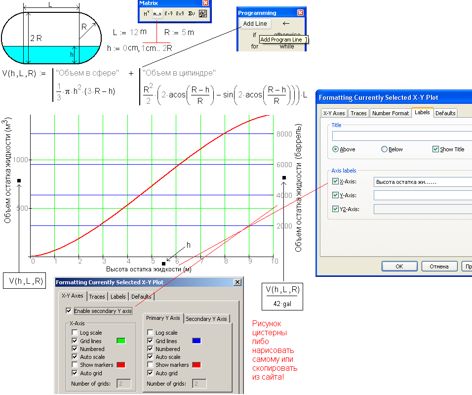
Fig. 1.67
shows the plot in which different y-axis represent different physical
quantities: the volume of the liquid layer and the square of its surface. We
may say that the essence the second y-axis is the second grid of y-axis (see Fig. 1.66 and 1.67). Earlier we could
represent two and more functions with single y-axis (up to sixteen) too (see
Fig. 1.64).
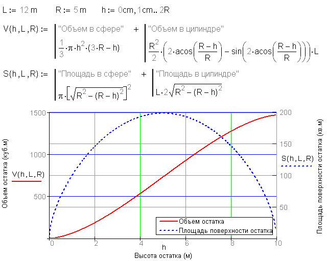
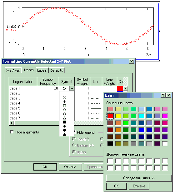
Besides, we
should remember of such a case. Here is a typical situation in mathematical
analysis: two plots are created in one coordinate system, a function and its
derivative. That could be considered as an error, which Mathcad is to interrupt
with such error message when meters are added with kilograms[30].
In addition, we can remind a problem from the book for intrants: find the
values of x of the given function in which this function is higher than its
derivative. For the reason that we cannot compare function and its derivative
because these values are different (the same meters and kilograms) the authors
say that “pure” mathematics does not connect a function and its derivative with
any physical quantities, for example with distance and speed. They also does
not agree to change the form of the problem but to keep the essence (derivation
and solving the unequality): to find values of x in which the derivative more
(less) than zero. From this it follows that we can draw two or more curves in a
single plot only if they are of the same dimension (length, time, force, etc).
Otherwise, a reader will apply himself to the meaning of their cross-points
while they have no meaning.
Often we
need to represent only definite combination of the arguments and functions. The
following example illustrates this thesis. The function returns the cost of a
used car depending of its age and run[31]
considering the mean speed (i.e. run divided by age) within the range from one
to two kilometers per hour. Fig. 1.68 shows that we insert the penalty into function Цена (Cost): if the real mean speed is out of that
range the function returns not the value but the text which is ignored on the
graph.
A
limitation of Mathcad 2D plotting is that variation range of the arguments must
be rectangular only. By default, the range is set square having spread in
values х and у from -5 to 5 and then a user
varying these numbers can make it rectangular. This range can be changed via
correspondent settings QuickPlot Data of the 3D Plot Format
dialog box but it is better to do it by function CreateMesh (see Fig. 1.69).
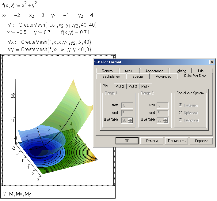
Function CreateMesh in Fig. 1.69 help us, first, to
draw the surface (semi-transparent) and level lines (lying on the x-y plane)
within the range determined by variables x1, x2, y1, and y2 and, second, to draw isolines by x and y axes that are in essence the surfaces pared down to the lines.
The variation
range can have complicated contour in the real problems. Here is an example
required non-rectangular variation range of the arguments in graphic solution
(Fig. 1.70).
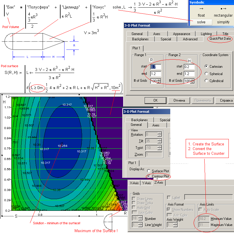
We need
to design outboard tank of a plane consisting from three parts (half-sphere,
cylinder, and cone), having definite volume, V=3 m3, with the minimum surface (the
typical optimization problem discussed in
The
limitation shown in Fig. 1.70 could be bypassed in the following way. If
the value of L (length
of the cylinder) becomes negative, function S returns not the complex number but zero. In
addition, we imposed a restriction to the problem: the ration of the tank
diameter to its length must be more than 0.5. After these restrictions (real L≥0 and forced 2R/(R+L+H)>0.5) had been inserted into function S its level lines became to were drawn
within non-rectangular (trapezium-shape) variation range R and H (non-rectangular variation range of the
function of two variables is discussed in
Fig. 1.71
shows the analytical solution of problem of optimal tank, the system of two
non-linear equations (partial derivatives of the function S with respect to arguments R and H) that returns 12 roots one of which (R=0.87776 and L=0.78512) is the coordinate of the “deepest
place” on Fig. 1.70.
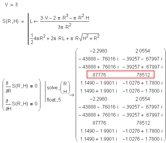
Fig. 1.72
shows other two methods from the large number of “ruses” which we need to draw the
graphs. To draw the graph of the type f(x,y)=0 we can remind that it is nothing
else than a zero level line of the contour graph of a function of two
arguments.
This
figure shows that “paying” with formats of 3D graph, turning it from surface (Surface
Plot) to level lines (Counter Plot) we can solve the problem both
regarding to Bernoulli’s lemniscate (upper graph) and more complicated closed
function (bottom graph) which cannot be factorized into definite functions and
plotted by the common technique.
Fig. 1.72
Fig. 1.72a Fig. 1.72b
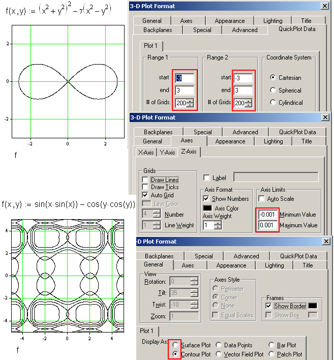
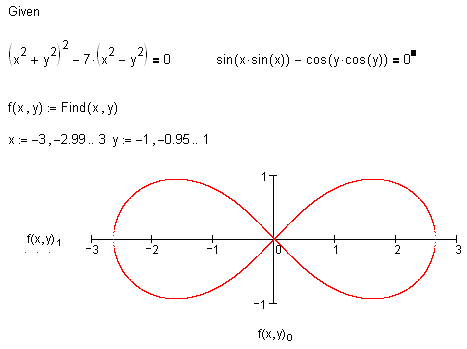
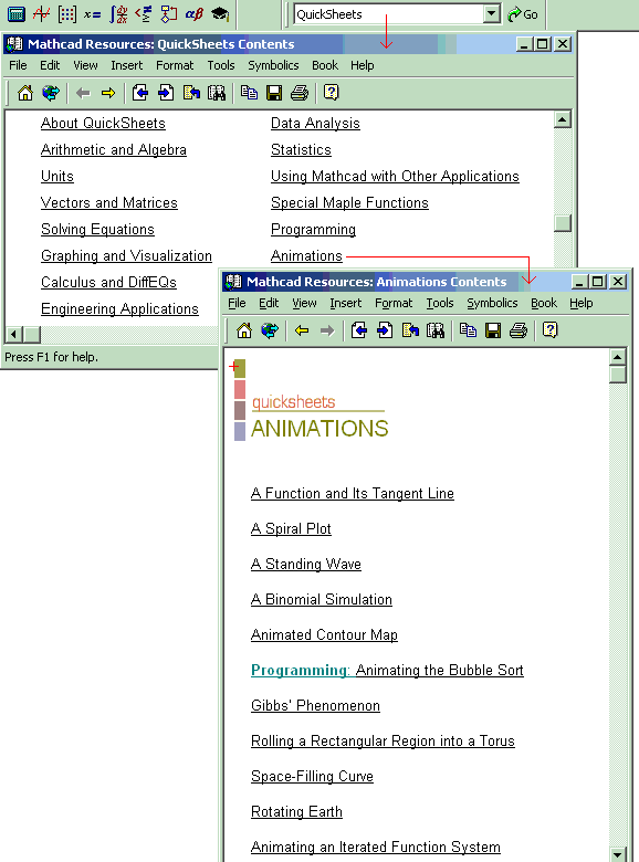
We
described only two ruses of formatting Mathcad plots (see Fig. 1.70 and
1.72). Nevertheless, there are much more of that especially in 3D plotting.
Often the graphs are formatted to transport to the books and articles as
PrintScreen. In that case, it is useful to insert the graph created in Mathcad
to another application, for example to Paint to finish it off. We have to do
that if Mathcad has not necessary formatting tools or they are difficult to
access, or we do not know about them.
1.7.
Animation and pseudo-animation
The
essence of animation in Mathcad and other applications can be explained on the
example of old children game. One draws a certain picture (a man in a
particular pose) on each page of a notebook changing a picture smoothly from
page to page. Turning the pages of such painted notebook, we shall not see the
animation effect. Although, pressing and turning it quickly, releasing by a
finger we can see the animation.
In
Mathcad, we can change manually the value of a variable and see changes of a
curve on a plot. Doing that quickly we cannot get animation, it is obtained
with the picture frequency not less than ten shot per second[33].
Therefore, Mathcad has special animation tools: predefined constant FRAME and two commands Record and Playback
from the Tools | Animation menu.
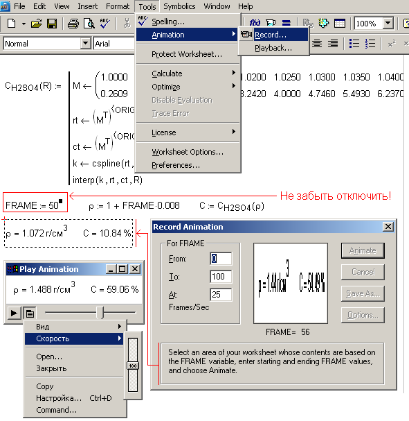
Fig. 1.73
shows the stages in creating animation in Mathcad in unusual way: to generate
peculiar exe-file. The function named CH2SO4is inserted into the Mathcad
worksheet which returns the concentration of sulphuric acid depending on its
density (by spline interpolation of the table values keeping in the matrix M –
the subject of
In the
end of 2003 Mathsoft Engineering & Education, Inc releases Mathcad
Application Server (MAS) for operation testing (see the description in
The guide
of Mathcad Application Server tells that the button Submit is useless in
the “standard” Mathcad worksheets but necessary in the WebSheets, Mathcad
worksheets converted to function as Web documents by MAS. This information is
inserted even in the Submit Button Properties dialog box.
Although,
this information (outlined in Fig. 1.74) confuses Mathcad users and cuts a
very interesting tool. First, we can manage without this button in WebSheets.
After the required changes were made we push the Submit button to
transmit that to the MAS server for computing in Mathcad installed in this
server. Although, if the inputs are changing only in Web Controls we can
format this “net” interface element so that its change and pushing
<Enter> results in sending the data on MAS-server without pushing the Submit
button which becomes unnecessary in this case.
Here we
can see analogy with manual mode in Mathcad (Excel, Word, BASIC, Pascal etc.)
and compare Submit button with
<F9> button which we press after the changes in the worksheet were
made by operator := and net and standard Controls and the calculation should be
done.
Second, Submit
button can be useful both in WebSheets and in worksheets, in traditional
Mathcad documents. The point is that pushing of this button increase by one
value of the variable connected with Submit (after starting Mathcad in any mode its value equals to one). This
variable is a peculiar counter of pushing the Submit button, i. e the
number of calling to MAS. This feature of Submit button can be very
useful in Internet and out of it: the formal variable can govern The Mathcad
worksheet changing it, for example. Thus, Fig. 1.75 show Mathcad worksheet
that illustrate the
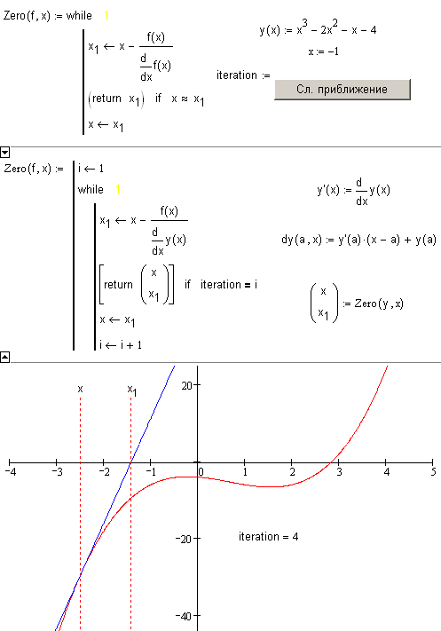
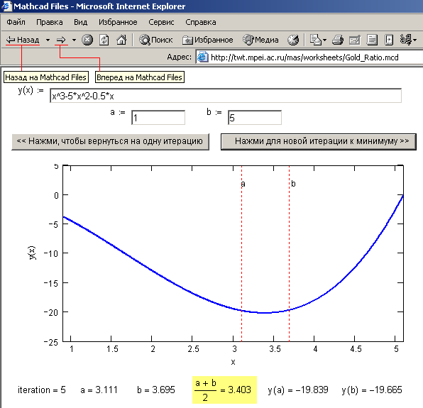
On the
author’s MAS server (www.vpu.ru/mas, section Разное) there are step by step illustrations
(pseudo-animation) of the following classic methods of numerical calculations
based on the Submit button:
r The
r The
r The method of halve in zero search
of a function — http://twt.mpei.ac.ru/MAS/Worksheets/secant.mcd;
r secant method in zero search of a
function — http://twt.mpei.ac.ru/MAS/Worksheets/secant.mcd;
r golden section in minimum search of
a function of one argument — http://twt.mpei.ac.ru/mas/worksheets/Gold_Ratio.mcd;
r Euler and Runge- Kutta methods with
constant interval of solving an ordinary differential equation — http://twt.mpei.ac.ru/mas/worksheets/Euler.mcd;
r Runge- Kutta method with variable
interval of solving an ordinary differential equation — http://twt.mpei.ac.ru/mas/worksheets/rkadapt.mcd;