11.2 The Rankine cycle
These shortcomings inherent in a steam power plant
realizing the Carnot cycle with wet steam can be partly remedied if heat is
rejected from the wet steam in the condenser before the entire steam condenses.
Thus, not wet steam with a small density but water is compressed from pressure
p2 to pressure p1 Compared to the specific volumes
of wet steam at point 3 (see
the T-s diagram in Fig.
11.2), the specific volume of water is small. Its compressibility is also
negligible compared with that of wet steam. Water is displaced from the
condenser into the boiler and its pressure is simultaneously increased not with
the aid of compressors but pumps of compact design, simple arrangement and
actuated by a rather low-power drive.
Such a cycle was suggested in the 1850's almost
simultaneously by the Scottish engineer and physicist W. Rankine and by R.
Clausius, and the cycle is usually called the Rankine cycle. The
schematic layout of a steam power plant operating on a Rankine cycle is similar
to the schematic layout depicted in Fig. 11.1, the only difference being that
in the Rankine cycle the 5 denotes a water pump and not a wet-steam
compressor.
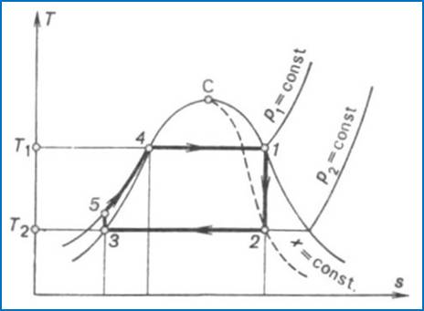
Fig. 11.4
Figure 11.4 shows the
Rankine cycle on a T-s diagram. In the condenser wet steam condenses
completely along the isobar p2 = const (point 3 in
Fig. 11.4). Water is then compressed in the pump from the pressure p2
to the pressure p1; this adiabatic process is represented
on the T-s diagram by the vertical line 3-5.
The length of line 3-5 is
small; as was already mentioned in Chapter 6, in the liquid region the isobars
are plotted on the T-s diagram very close to one another. Thus, when
water at a temperature of 25 °C and a saturation pressure of 3.1 kPa (0.032
kgf/cm2) is compressed isentropically to a pressure of 29 400 kPa
(300 kgf/cm2), water temperature rises by less than 1 °C, and we can
assume with a good degree of accuracy that in the liquid region the isobars for
water virtually coincide with the left boundary curve. Therefore, in plotting
the Rankine cycle on a T-s diagram, in the water region the isobars are
shown as merging with the left boundary curve.
The small length of adiabat
3-5 is evidence of the small amount of work expended by the pump to
compress the water.
It will be recalled that,
as was shown in Sec. 7.9, the work spent to compress the gas from pressure p2 to pressure p1
in a compressor is determined from relationship (7.188), which for 1 kg of working medium takes the following
form:
[since
v (p1) < v (p2), we have l21
< 0], and the work expended to realize the entire compressor cycle (the mechanical
work of compression) is determined from the formula

It will also be recalled that
for adiabatic compression, in accordance with Eq. (8.15),

where iout and iin are the enthalpies of the gas at the compressor
outlet (pressure p1) and before compression (pressure p2), respectively.
Equations (7.188) and (7.195a)
do not depend on the substance compressed; of course, the equations also hold
for the compression of liquid with the aid of a pump.
As a first approximation,
quite sufficient for technical calculations, water can be assumed as virtually
incompressible (vw =
const, i.e. dvw = 0) and,
consequently,

As to the mechanical work done by a pump, taking in
Eq. (7.195a) the quantity vw outside the integral sign,
we obtain:
 (11.1)
(the minus sign indicates
that work must be transferred to the pump from an external source of work).
The mechanical work done by a pump to compress
water is also small. For instance, if water is compressed from a pressure p2 = 3.1 kPa (0.032 kgf/cm2)
to a pressure p1 = 49 030 kPa (500 kgf/cm2),
according to Eq. (11.1), the work of the pump is

The same result can be obtained, using equation
(8.15). For this purpose, with the aid of an i-s diagram or Steam Tables, we
find the difference between the enthalpies of water on a given isentrop at
pressures p1 and p2.
The feed pump delivers water at a pressure pl to the boiler in which heat
is added isobarically at p1 = const. In the boiler
water is first heated to the boiling point (section 5-4 of the isobar p1 = const in Fig. 11.4) and
then vapourized (section 4-1 of the isobar p1 = const in Fig. 11.4). The
dry saturated vapour, generated in the boiler, passes into the turbine; the
process of steam expansion in the turbine is represented by the adiabat 1-2. The waste wet steam is
exhausted into the condenser and the vapour cycle closes.
From the viewpoint of
thermal efficiency the Rankine cycle seems to be less expedient than the
reversible Carnot cycle depicted in Fig. 11.2, inasmuch as the area ratio (just
as the average temperature of heat addition) is less for the former. However,
allowing for the practical conditions under which the cycle is to be realized
and also for the considerably smaller effect of the irreversibility of the
process of water compression, compared with the compression of wet vapour, on
the overall efficiency of a cycle, the Rankine cycle is more economical than
the corresponding Carnot cycle for wet steam. At the same time the replacement
of the cumbersome compressor, ensuring compression of the wet steam with a compact
feed water pump permits a substantial reduction in the costs involved in
building a steam power plant, and a simplification of its maintenance.
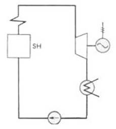
Fig. 11.5
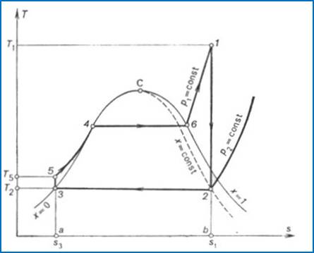
Fig. 11.6
Thus, the internal absolute
efficiencies of the two cycles will be approximately the same.
The thermal efficiency of
the Rankine cycle is increased by superheating the steam in a special
element of the steam boiler, the steam superheater (denoted SH in Fig.
11.5) in which steam is heated to a temperature exceeding the saturation
temperature at the given pressure p1. The T-s diagram
of the Rankine cycle with superheated steam is shown in Fig. 11.6. With
superheating the mean temperature of heat addition increases compared with the
temperature at which heat is added in a cycle without superheat. Consequently
the thermal efficiency of the cycle increases too.
It can be seen from Fig.
11.6 that in the Rankine cycle with superheat the process of steam expansion in
the turbine 1-2, realized up to the same pressure
as before, p2, ends inside the two-phase region at a dryness
fraction higher than in the cycle depicted in Fig. 11.4. Because of this, the
turbine blading operates under lighter conditions and, consequently, there is
an increase in the internal relative efficiency of the turbine and in the
internal efficiency of the cycle  ; for a cycle with superheat the efficiency
increases both because of an increase in
; for a cycle with superheat the efficiency
increases both because of an increase in  and in the
internal relative efficiency
and in the
internal relative efficiency  .
.
The Rankine cycle with
superheat is the basic cycle for thermopower plants with application in
up-to-date heat and power engineering.
The quantity of heat added
to the working medium in the cycle, q1, is represented on
the T-s diagram shown in
Fig. 11.6 by the area a-3-5-4-6-l-b-a. The heat rejected in the cycle, q2,
is equivalent to area a-3-2-b-a, and the work output of the cycle,
to area 3-5-4-6-1-2-3.
Since in the Rankine cycle
the processes of heat addition and rejection are isobaric, and in an isobaric
process the quantity of heat added (rejected) is equal to the difference
between the enthalpies of the working medium at the beginning and end of the
cycle, as applied to the Rankine cycle, we can then write
 (11.2)
 (11.3)
(the
subscripts for i correspond to
the notations of the state of the working medium used in Fig. 11.6).
Here, i1 is
the enthalpy of superheated water vapour (steam) at the exit of the boiler (at a pressure p1 and a
temperature T1); i5 is the enthalpy of water at the boiler
inlet, i.e. at the pump outlet (at a pressure p1 and a temperature
T6); i2 is the enthalpy of wet
steam at the turbine exit (exhaust steam), i.e. at the condenser inlet (at a
pressure p2 and with a dryness fraction x); and i3
is the enthalpy of water at the condenser outlet (equal to the enthalpy of
water on the saturation line, i', at
the saturation temperature T2 determined
directly by pressure p2).
Taking the above
relationship into account, from the general expression for thermal efficiency
of a cycle,

applied
to the reversible Rankine cycle we have:
 (11.4)
This equation can be presented in the following
form:
 (11.4a)
The difference  represents
the available enthalpy drop converted into the kinetic energy of flow and then,
into work in the turbine. In accordance with Eq. (8.15), the difference
represents
the available enthalpy drop converted into the kinetic energy of flow and then,
into work in the turbine. In accordance with Eq. (8.15), the difference  represents
the mechanical work of the pump. Thus, the work of the cycle can be considered
as the difference between the work done in the turbine and the work expended
to drive the pump.
represents
the mechanical work of the pump. Thus, the work of the cycle can be considered
as the difference between the work done in the turbine and the work expended
to drive the pump.
If we introduce the
following notations:
 (11.5)
and
 (11.6)
then
 (11.7)
the superscripts "theor" and
"r" indicate that these quantities pertain to a theoretical
reversible cycle, not accounting for losses due to the irreversibility of real
processes.
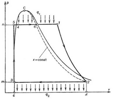
Fig. 11.7
The quantity  should not be confused with the work of expansion,
and
should not be confused with the work of expansion,
and  with the work of compression in a cycle. The
Rankine cycle is represented on the p-v
diagram in Fig.
11.7 (the notations are the same as in Fig. 11.6). On this diagram the isobar 5-4-6-1 (p1 =
const) represents the addition of heat in the cycle, line 1-2 shows
adiabatic expansion of steam in the turbine, line 2-3 is the isobar (p2
= const) along which heat is rejected in the condenser, and line 3-5
represents the adiabatic compression of water in the pump (due to the small
compressibility of water, this adiabat practically coincides with an isochor).
As can be seen from this diagram, the work of expansion is equal to the area c-5-l-2-d-c,
the work of compression to the area c-3-2-d-c, and the work output
of the cycle is represented by area 1-2-3-5-1.
with the work of compression in a cycle. The
Rankine cycle is represented on the p-v
diagram in Fig.
11.7 (the notations are the same as in Fig. 11.6). On this diagram the isobar 5-4-6-1 (p1 =
const) represents the addition of heat in the cycle, line 1-2 shows
adiabatic expansion of steam in the turbine, line 2-3 is the isobar (p2
= const) along which heat is rejected in the condenser, and line 3-5
represents the adiabatic compression of water in the pump (due to the small
compressibility of water, this adiabat practically coincides with an isochor).
As can be seen from this diagram, the work of expansion is equal to the area c-5-l-2-d-c,
the work of compression to the area c-3-2-d-c, and the work output
of the cycle is represented by area 1-2-3-5-1.
The quantities
and are
represented on the p-v diagram
in the following manner. In accordance with Eq. (8.15),  is represented by area 1-2-m-n-l. Equation
(7.195a) indicates that the difference
is represented by area 1-2-m-n-l. Equation
(7.195a) indicates that the difference  is represented by area 5-3-m-n-5. It follows
that the work output of the cycle, equal to the
difference
is represented by area 5-3-m-n-5. It follows
that the work output of the cycle, equal to the
difference  is represented by area 1-2-3-5-1.
Taking into account Eq. (11.1) for the mechanical
work performed by the pump,
 (11.8)
for relationship (11.4a) we have:
 (11.9)
Equations (11.4a) or (11.9)
make it possible to determine with the aid of an i-s diagram or
Steam Tables the thermal efficiency of the reversible Rankine cycle in terms of
the known initial parameters of the steam (i.e. the steam pressure p1
and temperature T1 at
the turbine inlet) and the steam pressure p2 in the
condenser.
Thus,
if the initial steam conditions are pressure p1 = 16 670 kPa
(170 kgf/cm2) and temperature T1 = 550 °C, and
condenser pressure is maintained equal to p2
= 4 kPa (0.04
kgf/cm2), the magnitude of the thermal efficiency η is calculated in the following
way. From the Steam Tables we
find that at a pressure of 16 670 kPa (170 kgf/cm2) and a
temperature of 550 °C the enthalpy of steam is i1 =
3438 kj/kg (821.2 kcal/kg), the entropy of steam s1 = 64 619
kJ/(kg-K) [15 434 kcal/(kg-K)]. Now an i-s diagram is used to find the
enthalpy of wet steam i2
at a pressure p2 = 4 kPa
(0.04 kgf/cm2) and the same as at point 1, value of entropy (in
a reversible process the expansion adiabat coincides with an isentrop). This
enthalpy is i2 = 1945
kj/kg (464.5 kcal/kg).
The
enthalpy of water on the saturation line at a pressure p2 = 4
kPa (0.04 kgf/cm2) is
i3 = 120 kj/kg
(28.7 kcal/kg). The entropy of water in this state is equal to 0.4178 kJ/kg-K
[0.0998 kcal/(kg-K)]. From the Steam Tables we find the value of the enthalpy
of water at point 5 (the pump exit) at a pressure 16 670 kPa (170 kgf/cm2)
and at the same value of the entropy as at point 3: i5 = 137 kj/kg (32.7 kcal/kg); the temperature of water
T5 = 29 °C.
Thus,
=
1493 kJ/kg (356.7 kcal/kg); =
17 kJ/kg (4.0 kcal/kg);
 = 3301 kJ/kg (788.5 kcal/kg). Substituting
these values into Eq. (11.4a), we obtain the thermal efficiency of this
reversible Rankine cycle, η =
0.46. It will be indicated for the sake of comparison that the thermal
efficiency of a reversible Carnot cycle realized in the same temperature
interval (550 °C to 28.6 °C) is
= 3301 kJ/kg (788.5 kcal/kg). Substituting
these values into Eq. (11.4a), we obtain the thermal efficiency of this
reversible Rankine cycle, η =
0.46. It will be indicated for the sake of comparison that the thermal
efficiency of a reversible Carnot cycle realized in the same temperature
interval (550 °C to 28.6 °C) is  = 0.63, much greater
than the thermal efficiency of the reversible Rankine cycle calculated above.
= 0.63, much greater
than the thermal efficiency of the reversible Rankine cycle calculated above.
Figure 11.8 shows the
Rankine cycle on an i-s diagram (the notations are the
same as on the T-s and p-v diagrams shown in
Figs. 11.6 and 11.7). It is clear, in accordance with Eq. (11.4a), that on this
diagram the distance along the i-axis
between points 1 and 2 corresponds to the work done by the
turbine, the distance between points 5 and 3 represents the work expended
in the pump, the distance between points 1 and 5 represents the
heat q1 added in the cycle, and the distance between points 2
and 3 shows the amount of heat q2 rejected in the
cycle.
If the work done by the
pump, , is negligible compared with the drop in enthalpy
in the turbine, , i.e. if we consider that i3 = i5, then Eq. (11.4a) can be presented in the following
form:
 (11.10)
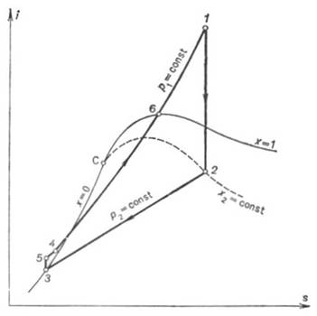
Fig. 11.8
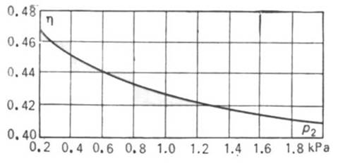
Fig. 11.9
This relationship is quite suitable for estimating
calculations of low-pressure steam power cycles. When dealing with
high-pressure steam power plants the work of the pump cannot be ignored.
Let us find the dependence
of the thermal efficiency of the Rankine cycle on the initial conditions of the
steam.
Under the same initial steam conditions (p1 and T1)
a decrease in condenser pressure p2 leads to a higher
thermal efficiency: inasmuch as in the two-phase region pressure is directly
related with temperature, a decrease in p2 means a decrease of the
temperature at which heat is rejected in the cycle, T2. Thus, the temperature interval of the cycle
widens and the thermal efficiency rises.
The nature of the dependence of thermal efficiency η on condenser pressure p2
is illustrated graphically in Fig. 11.9. This graph is plotted for the
above cycle realized with initial steam conditions p1 =16670 kPa (170 kgf/cm2)
and T1=550°C;
the values of the thermal efficiency are calculated with the aid of Eq.
(11.4a).
In modern steam power plants
condenser pressure p2, usually
predetermined by the temperature of the condenser cooling water, is 3.5 to 4.0
kPa (0.035 to 0.040 kgf/cm2); a pressure of 4.0 kPa (0.04 kgf/cm2)
corresponds to a saturation temperature T2
=28.6°C. A further reduction of condenser pressure
is inexpedient. First, a greater rarefaction (vacuum) causes the specific
volume of the exhaust steam flowing into the condenser from the turbine to
increase, requiring a larger condenser and much longer blades in the last turbine stages. Second, a greater
rarefaction causes the temperature of the wet steam in the condenser to
decrease (for a pressure of 3.0 kPa the water saturation temperature is 23.8°C,
and for a pressure of 2.0 kPa it is 17.2 °C), resulting in a very small difference
between the temperatures of the condensing steam and the condenser cooling
water
to which the condenser's external surfaces are exposed, requiring a larger
condenser.
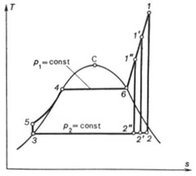
Fig. 11.10
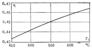
Fig. 11.11
However, the thermal
efficiency of the Rankine cycle depends above all on the initial steam
condition, p1 and T1
.With a rise in superheat temperature T1 at the same
pressure the thermal efficiency of the cycle increases, since there is a higher
mean temperature of heat addition in the cycle, as illustrated in Fig. 11.10.
To illustrate, Fig. 11.11 shows a graph on which the thermal efficiency is
plotted against T1 for
a Rankine cycle in which the initial steam pressure p1 = 16 670
kPa (170 kgf/cm2), and the pressure of steam in the condenser p2
= 4.0 kPa (0.04 kgf/cm2). If T1 is constant, an increase in the pressure p1 also leads to a rise of
the thermal efficiency of the cycle; the higher the p1 the
greater the cycle areas ratio and the higher the mean temperature of heat
addition (Fig. 11.12).
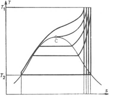
Fig.
11.12
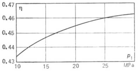
Fig.
11.13
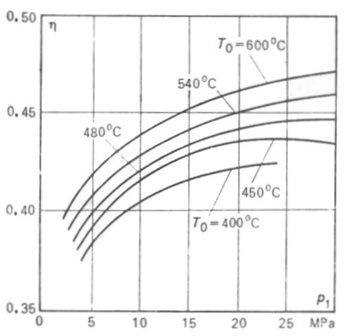
Fig.
11.14
However, with rising p1
at the same superheat temperature, the wetness of exhaust steam (at the
turbine exit) increases involving a drop in turbine relative internal
efficiency. Therefore, when raising the initial steam pressure, it is also
desirable to increase the throttle steam temperature. In Fig. 11.13 the thermal
efficiency of the Rankine cycle is plotted against p1 at a superheat
temperature T1 = 550 °C and p2 = 4.0 kPa
(0.04 kgf/cm2).
It is clear that the higher
the steam pressure p1 and temperature T1, the higher the thermal
efficiency of the Rankine cycle. In Fig. 11.14 the thermal efficiency η of the reversible Rankine cycle
is plotted against p1.
Thus, to raise the thermal efficiency of a Rankine
cycle, in principle an attempt should be made to raise the initial steam
conditions.
At present the basic initial steam conditions
practiced in Russian electric power stations are p1 = 23 500
kPa (240 kgf/cm2) and T1 = 565 °C. Pilot plants
are being operated with steam conditions p1 = 29 400 kPa (300
kgf/cm2) and a throttle steam temperature up to T1 = 650
°C.
A further increase in the initial
steam conditions is restricted by the properties of the construction materials
presently available: at high pressures and temperatures the strength of
pearlitic grades of steel deteriorates, and they must be replaced with
considerably more expensive austenitic steels. Although such a change permits
operation at higher p1 and T1, resulting in
a somewhat higher thermal efficiency of the cycle, investments increase. In
other words, although fuel is saved, more expensive metals are consumed.
Considering the problem from this viewpoint, a further increase in initial
steam conditions is inexpedient, especially where cheap grades of fuel are
available. This problem is solved on the basis of a comprehensive technical and
economic analysis.