3.6 Entropy
Let us turn now to consider some essential properties of reversible
cycles. The thermal efficiency of a reversible Carnot cycle is found from the
relationship
![]()
In the
most general form, by definition, the thermal efficiency of any cycle
![]()
from which it follows that for a reversible Carnot cycle
![]() (3.107)
(3.107)
or, which is the same,
![]() (3.108)
(3.108)
In the general form Eq. (3.108) becomes[1]
![]() (3.109)
(3.109)
Equation (3.109) can be presented in the form
![]() (3.110)
(3.110)
Consider an arbitrary reversible cycle. It will be recalled that to
accomplish an arbitrary reversible cycle an infinite number of heat sources must
be available. It will also be recalled that, as it was made clear in Sec. 3.4,
any reversible cycle can be visualized as consisting of a multitude of elementary
Carnot cycles (Fig. 3.8), each of which is associated with a high-temperature
source from which it receives heat ΔQ1
and with a low-temperature source to which it transfers heat ΔQ2.With account taken of Eq.
(3.109), we can write for each of these elementary cycles (denote their total
number by n):
1st cycle ![]()
2nd cycle ![]()
.…………………..
nth cycle ![]()
Adding
these relations, we obtain:
![]() (3.111)
(3.111)
or, by analogy with Eq. (3.110),
![]() (3.112)
(3.112)
In the limit, if infinitely small cycles are considered,
![]() (3.113)
(3.113)
whence, is accordance with Eq. (3.112), we obtain:
![]() (3.114)
(3.114)
The integral in Eq. (3.114) is called the Clausius integral. Equation (3.114) shows that for
any reversible cycle the Clausius integral is equal to zero. Let us elucidate the properties of the integrand. Denote
it by
![]() (3.115)
(3.115)
Upon substitution, Eq. (3.114)
reduces to
![]() (3.116)
(3.116)
It can be readily shown that the magnitude of the integral along any
closed path, between two arbitrary states A and B as limits (Fig.
3.12) does not depend on the path of the process, but depends on the final
states, i.e.
 (3.117)
Thus, the integrand S,
similar to interval energy and enthalpy, is a function of state, and
its magnitude is determined unambiguously by the properties (parameters) of
state. It will also be recalled that as it was mentioned in Sec. 2.4, the
differential of a function of state is a
total differential.

Fig. 3.12
Heat (just as
work) is a function of the process, and the amount of heat added to, or removed
from, a system depends on the path of the process. Similar to any function of
the process, the differential of the amount of heat, dQ, is not a total differential[2].
On the other hand, it follows from the foregoing that being multiplied by the
quantity 1/T, this
differential dQ turns into a total
differential dS = dQ/T. Thus, the
quantity 1/T is an integrating
factor for the differential of the amount of heat (it will be recalled that in
mathematics by an integrating factor is meant a function µ such that after
multiplication by this factor the quantity dX, which is not a total differential,
turns into a total differential dY = µdX; it is known from mathematics that
in the event of two variables, it is possible to find an integrating factor for
any expression that is not a total differential.
The function S introduced by Clausius is called the entropy.
Entropy is an extensive property and, similar to other extensive
quantities, it possesses the property of additivity. The quantity
![]() (3.118)
(3.118)
is referred to as specific entropy, and is defined as
the entropy of a unit mass of substance.
Just like any other function of state, the specific entropy of a system
can be presented as a function of any two properties of state, x and y:
![]() (3.119)
(3.119)
where p and v, p and T,
etc., can be present as x and y.
The methods used to calculate the entropy of a substance with the aid of
other thermal quantities will be treated in detail in Chapters 4 and 6.
The definition of entropy (3.115) makes it clear that entropy is
measured in units of heat divided by temperature. The most commonly used units
of entropy are J/K.
The units of specific entropy are J/(kg·K), kJ/(kg·K), sometimes
kcal/(kg·K) and etc. Thus, the unit of measurement of
entropy coincides with that of heat capacity. For a pure substance and for a
mixture of substances not reacting chemically with each other the zero for
entropy can be chosen arbitrarily, just as the zero for internal energy. In
considering various thermodynamic processes, we will be interested in the
change of the entropy involved in these processes, i.e. the difference between
the entropies at the initial and final points of the processes, which,
naturally, depends in no way on the entropy zero point.
It is clear from definition (3.115) that in various reversible processes
the entropy of a system can either increase or diminish: inasmuch as temperature
T is always positive, from equation (3.115) it follows that when heat is
added to the system (dQ > 0), its entropy increases (dS >
0), and when heat is removed from the system (dQ < 0), its entropy
decreases (dS
< 0). It follows from Eq. (3.115) that when in a reversible
process a body undergoes a change from the initial state 1 to the final state
2, the entropy of the body changes by
![]() (3.120)
(3.120)
Calculate, for example, the change in the entropy of 10 kg of water
heated from a temperature of T1
= 20 °C to a temperature T2 = 60 °C at atmospheric pressure; in
this temperature interval the heat capacity of water is assumed at first
approximation to be independent of temperature and equal to 4.19 kJ/(kg·K). Since
![]()
we take G and cp out of the
integral, and from Eq. (3.120) we get:
![]()
or
![]()
One important fact should be specially emphasized. The concept of entropy
was introduced by investigating reversible cycles. This would seem to make it
impossible to investigate the concept of entropy in the analysis of irreversible
processes. But it must be borne in mind that entropy is a function of state
and, consequently, the change of entropy in any process is only defined by the
final and initial states.
The concept of entropy permits the introduction of the temperature-entropy
chart, or diagram, in which entropy is plotted along the abscissa, and absolute
temperature along the ordinate (Fig. 3.13). This chart facilitates to a great
extent the analysis of heat engines. Let us plot the curve (path) of an
arbitrary process on the T-S
diagram.
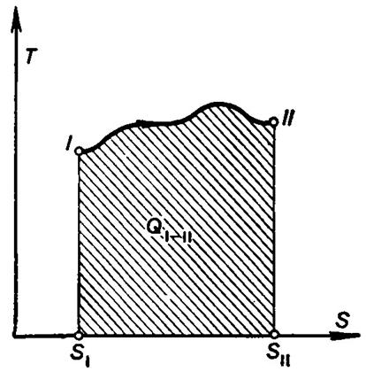
Fig. 3.13
From Eq. (3.115) it follows that in a reversible process
![]() (3.121)
(3.121)
The amount of heat added to a system (or removed from it) in a
reversible process between the states I
and II is:
 (3.122)
It is clear that the amount of heat received (rejected) by a system in a
reversible process will be represented on the T-S diagram by the area under the path of the process.
Fig. 3.14 shows a reversible cycle of a heat engine on a T-S diagram. The amount of heat
Q1 added to the working
medium in the cycle is represented by the area under the curve ABC, and the amount of heat Q2 removed from the
working medium is represented by the area under the curve CDA. The work done by the working medium
in the cycle, Lc
= Q1 - Q2, is represented on the
diagram by the area confined by the closed curve ABCDA.
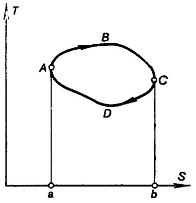
Fig. 3.14
The T-S diagram is convenient since it gives a visual
presentation of the amount of heat added and removed (rejected) in a cycle and
the work obtained due to the accomplished cycle (or the work expended if a
reverse cycle is involved). The T-S
diagram also shows where in the process heat is added to the working body and where heat is removed from it: the
process of reversible addition of heat is characterized by an increase in
entropy, and the process of heat removal by a decrease.
An isothermal process is evidently represented on the T-S diagram
by a horizontal straight line.
It follows from Eq. (3.122) that in the isothermal process
![]()
It is clear from equation
![]()
that in a reversible adiabatic process (dQ =
0)
![]() (3.123)
(3.123)
or
![]() (3.124)
(3.124)
That is why reversible adiabatic processes are also referred to
as isentropic, and the
path of such a process is called an isentropic, which in the T-S
diagram is represented by a vertical line.
It ought to be noted that in the T-S diagram, just as in any other thermodynamic diagram of
state, only reversible equilibrium processes can be plotted.
A reversible Carnot cycle is represented on the T-S diagram by the rectangle 1-2-3-4-1 (Fig.
3.15), bounded by isotherms 1-2
(T1 = const)
and 3-4 (T2
= const) and by reversible adiabats
2-3 (S2
= const) and 4-1
(S1 = const).
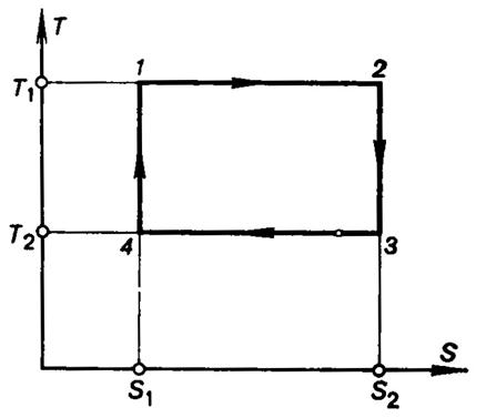
Fig. 3.15
The amount of heat added in this cycle to the working medium from the
high-temperature heat source,
![]() (3.125)
(3.125)
is represented on the diagram by rectangle 1-2-S2-S1-1;
the amount of heat transferred to the low-temperature source,
![]() (3.126)
(3.126)
by the rectangle 3-S2-S1-4-3; and the work output of
the cycle,
![]()
is represented by rectangle 1-2-3-4-1.
From the general expression for the thermal efficiency
of a cycle, and with account taken of Eqs. (3.125) and
(3.126), for a reversible Carnot cycle we obtain:
![]()
or, which is the same,
![]()
which coincides with Eq. (3.32), as was to be expected.
The T-S diagram has made it possible to prove easily the validity
of the following statement:
The thermal efficiency of any reversible cycle realized between more
than two heat sources is less than the efficiency of a reversible Carnot cycle
realized between the same limiting temperatures.
Compare the arbitrary reversible cycle I with the Carnot cycle II
that operates in the same temperature interval of cycle I (Fig. 3.16). Plot the Carnot cycle 1-2-3-4 around cycle I, and give the Carnot cycle the name III. Then
![]() (3.127)
(3.127)
![]() (3.128)
(3.128)
whence it follows that
![]() (3.129)
(3.129)
Thus, within a given temperature interval the thermal efficiency of a
reversible Carnot cycle is greater than the thermal efficiency of any other
reversible cycle. The reversible Carnot cycle is, consequently, a kind of a
standard, enabling to determine the effectiveness of any other cycle operated
in the same temperature interval, by comparing the thermal efficiency of this
cycle with that of the Carnot cycle. This is the special importance of Carnot
cycle, distinguishing it among any other cycles of heat engines.
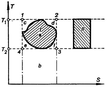
Fig. 3.16
The greater any arbitrary cycle fills the rectangle representing the
reversible Carnot cycle, operated in the same temperature interval and in the
same interval of entropies (as it is said, the higher the cycle-filling
coefficient or the area ratio of a cycle), the higher the thermal
efficiency of this arbitrary reversible cycle is. The cycle of any heat engine
should be organized so that the area ratio of this cycle is as large as
possible.
Let us turn now to the analysis of one more important variety of cycles
of heat engines. Consider the reversible cycle, represented on the T-S diagram in Fig. 3.17 and
consisting of two isotherms and two arbitrary equidistant curves.
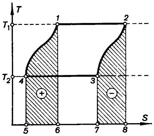
Fig. 3.17
The curves 4-1 and 2-3 are equidistant, and to accomplish
the reversible processes corresponding to these curves there should be
available an infinitely large number of heat sources.
During the process 2-3 heat is removed from the working medium (-)
in an amount determined by the area 2-8-7-3-2 and equal to the heat
added to the working medium during the process 4-1 and determined by the
equal area 1-6-5-4-1. The heat sources can be replaced by so-called
regenerators, which during the process 6-1 reject the amount of heat
(and at the same temperatures) returning to them from the working medium during
the process 2-3. The cycle results in that each of the infinitely large
number of heat regenerators neither rejects nor receives heat on the whole. The
heat added to the working medium in the cycle, Q1 = T1 (S2 – S1), is represented by the area 1-2-8-6-1, and the heat rejected in the
cycle, Q2 = T2 (S3
- S4), by the area 3-7-6-5-4-3.
In consequence of the curves 4-1 and 3-2 being equidistant,
![]()
whence
![]()
The cycle considered above is known as the cycle with complete
regeneration of heat, or the regenerative cycle. The regenerator effectiveness, determined by the ratio
of the area (+) to the area (-), is equal to unity in this cycle, with a
regenerator effectiveness less than unity the cycle is said to be a cycle with
incomplete regeneration. An increase in the regenerator effectiveness brings
this cycle closer to the Carnot cycle, and in the limit, as it can be seen from
the case considered, ![]()
Thus, the thermal efficiency of any reversible cycle, accomplished
between two heat sources (i.e. a regenerative cycle), is equal to the thermal
efficiency of the reversible Carnot cycle operated in the same temperature
interval.
Incomplete heat regeneration also increases the thermal efficiency of
any (both reversible and irreversible) cycles, since regeneration always
increase the area ratio of a cycle.