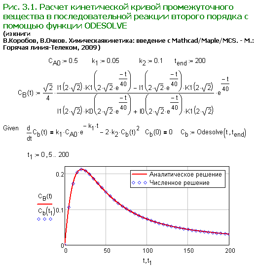
Fig. 3.1.

Kinetic curve calculation for an intermediate in a consecutive second-order reaction using Odesolve function

png

MC11

MC13

MC14-15

MCS

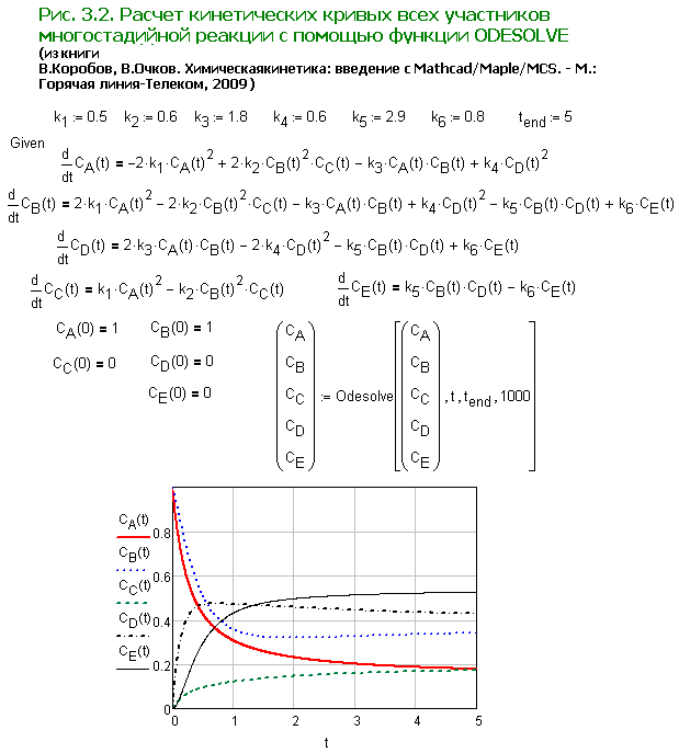
Fig. 3.2.

Calculation of the kinetic curves for all components in a multi-step reaction using ODESOLVE function

png

MC11

MC13

MC14-15

MCS

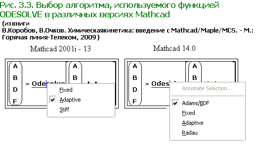
Fig. 3.3

Choosing an ODESOLVE algorithm in different Mathcad versions

png

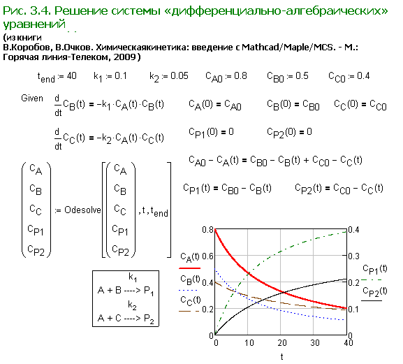
Fig. 3.4.

Solving a system of "differential—algebraic" equations

png

MC14-15

MCS

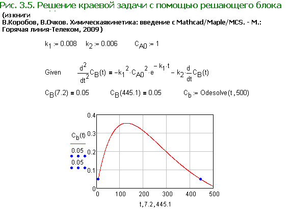
Fig. 3.5.

Solving a boundary-value problem with solver

png

MC11

MC13

MC14-15

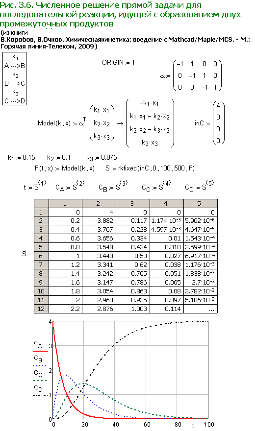
Fig. 3.6.

Numerical solution of the direct problem for a consecutive reaction with two intermediates

png

MC11

MC13

MC14-15

MCS

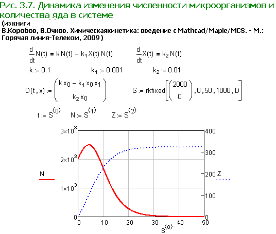
Fig. 3.7.

Microorganism population and poison amount trends

png

MC11

MC13

MC14-15

MCS

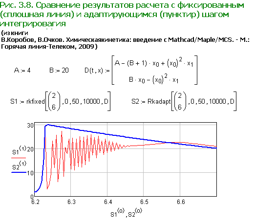
Fig. 3.8.

Comparison of the results for calculations with fixed step of integration

png

MC11

MC13

MC14-15

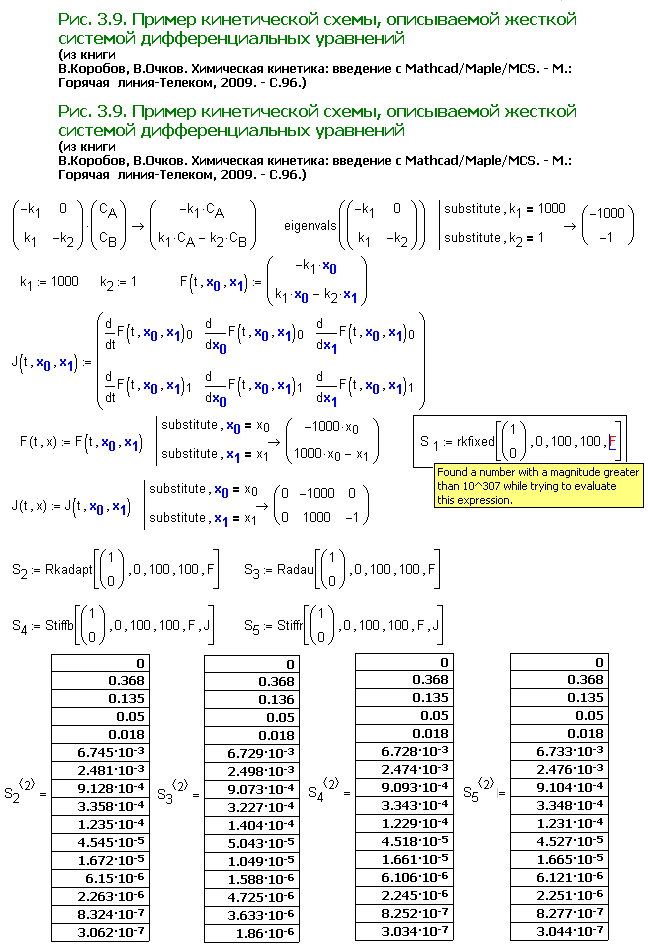
Fig. 3.9.

An example of a kinetic scheme described with a stiff set of differential equations

png

MC11

MC13

MC14-15

MCS

Fig. 3.10.

Numerical solution of the direct kinetic problem using Mathcad tools

png

Maple 9

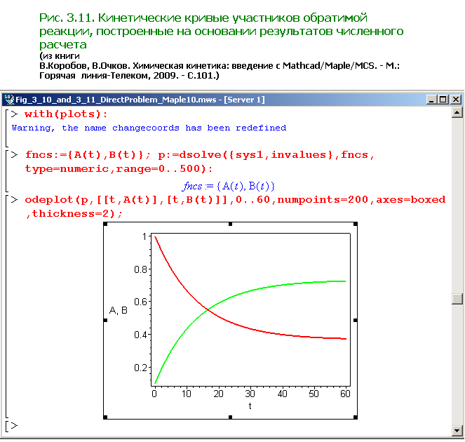
Fig. 3.11.

Kinetic curves for reversible reaction participants calculated using numerical calculation results

png

Maple 9

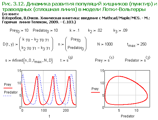
Fig. 3.12.

Population trends for predators (dashed line) and prey (solid line) in the
Lotka–Volterra model

png

MC11

MC13

MC14-15

MCS

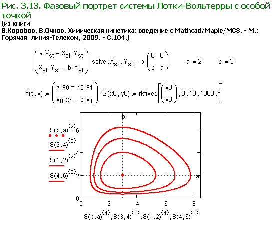
Fig. 3.13.

Phase portrait of the Lotka—Volterra system with a critical point

png

MC11

MC13

MC14-15

MCS

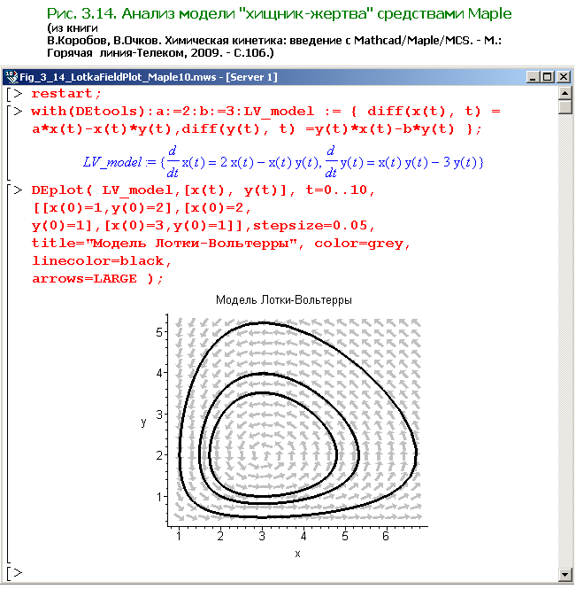
Fig. 3.14.

"Predator—prey" model analysis using Maple

png

Maple 9

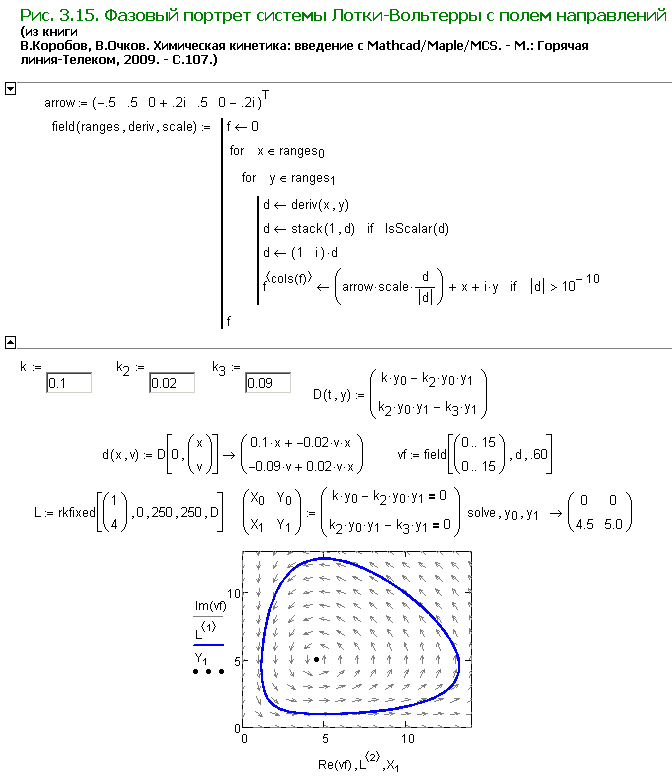
Fig. 3.15.

Phase portrait of the Lotka—Volterra system using a directional field

png

MC11

MC13

MC14-15

MCS

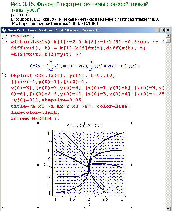
Fig. 3.16.

Phase portrait of the system with "node"−type critical point

png

Maple 9

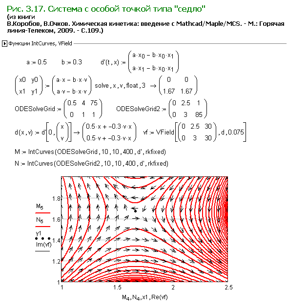
Fig. 3.17.

System with a “saddle” critical point

png

MC11

MC13

MC14-15

Fig. 3.18.

Modelling the photosynthesis kinetics

png

MC11

MC13

MC14-15

MCS

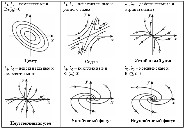
Fig. 3.19.

Possible critical point types and phase portraits versus different Jacobian
matrix eigenvalues

png

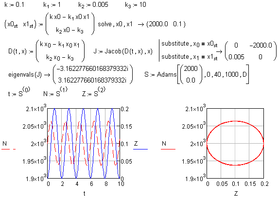
Fig. 3.20.

Oscillation mode of the population trend in microorganism colony

png

MC11

MC13

MC14-15

MCS

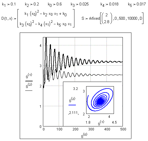
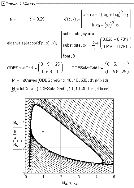
Fig. 3.21.

Brusselator phase portrait with a limit cycle

png

MC11

MC13

MC14-15

MCS

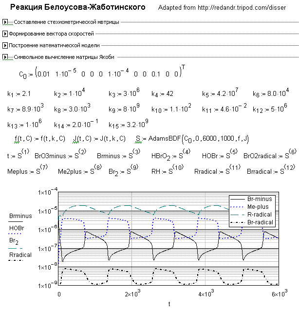
Fig. 3.22.

Concentration oscillations in the Belousov–Zhabotinsky reaction

png

MC14/15

MCS

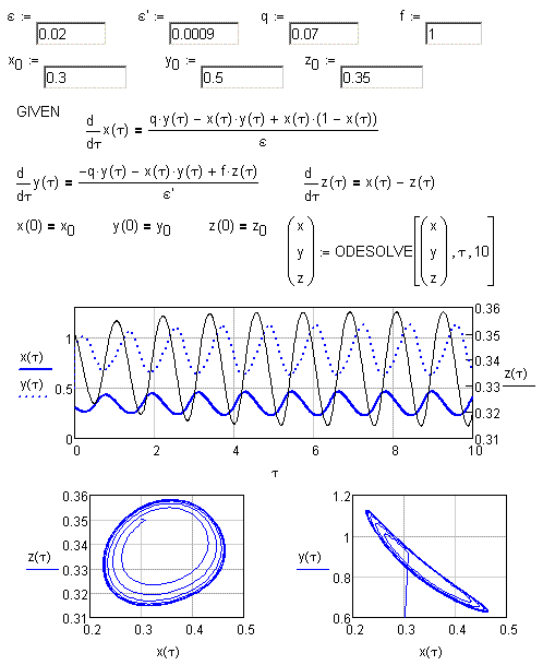
Fig. 3.23.

One of the direct problem solutions for the oregonator problem

png

MC11

MC13

MC14/15

MCS

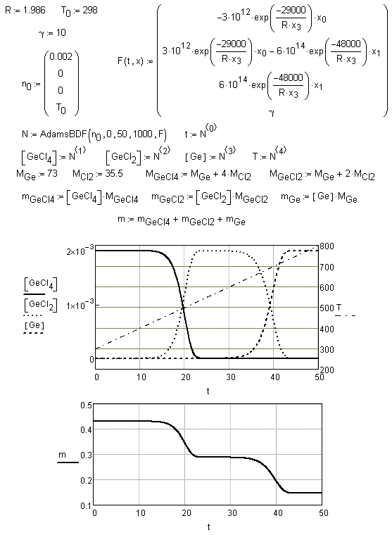
Fig. 3.24.

Solution of the GeCl₄ decomposition problem

png

MC11

MC13

MC14-15

MCS

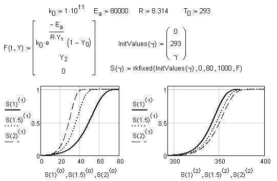
Fig. 3.25.

Conversion vs. time and temperature for different heating rates

png

MC11

MC13

MC14

MCS

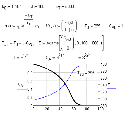
Fig. 3.26.

Temperature and reagent concentration changes in a periodic adiabatic
reactor

png

MC11

MC13

MC14

MCS

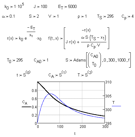
Fig. 3.27.

Operation dynamics of a periodic nonadiabatic reactor

png

MC11

MC13

MC14

MCS

Fig. 3.28.

Temperature and concentration trends in a flow adiabatic reactor

png

MC11

MC13

MC14

MCS

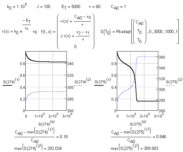
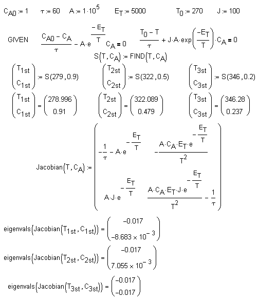
Fig. 3.29.

Computations of possible stationary states and analysis of their
stability

png

MC11

MC13

MC14

MCS

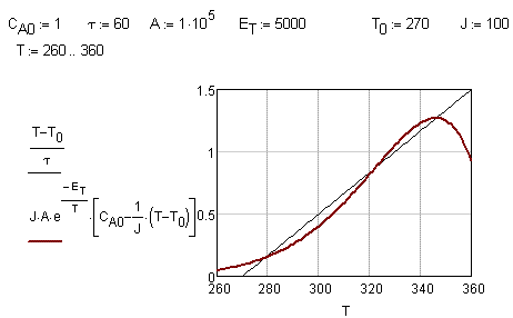
Fig. 3.30.

Graphical representation of possible stationary states

png

MC11

MC13

MC14

MCS

Fig. 3.31.

Phase portrait for exothermic reaction in an adiabatic flow reactor

png

MC11

MC13

MC14

MCS