"Differential models.
An Introduction with Mathcad”
Springer Publishing House (Springer-Verlag, 2004, ISBN: 3-540-20852-6)
WebSheets of the book (Mathcad Application Server)
Chapter 1. Differential mathematical
models
1.1. Introduction
1.2. Laws in the Differential Form
1.3. Models of Growth
1.4. Conservation Laws
1.5.
Conclusion
Chapter 2. Integrable differential equations
2.1. List of Integrable Equations
2.2. First-Order Linear Equations
2.3. Linear Homogeneous Equations with Constant Coefficients
2.4. Linear Inhomogeneous Equations
2.5. Equations with Separable Variables
2.6. Homogeneous Differential Equations
2.7.
Depression of Equation
Chapter 3. Dynamic model of the system
with heat generating
3.1.
Introduction
3.2. Mathematical Model
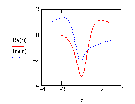
3.3. Phase-Plane Portrait. Stable and Unstable Equilibrium
3.4. State Set Representation
3.5. Plotting of Bifurcation Set
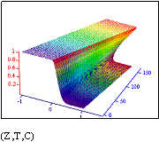
3.6. Three-Dimensional State Set Representation in the Form of
the Fold
Catastrophe
3.7. Catastrophic Jumps at Smooth Variation of Parameters
3.8. Time Evolution of System with Heat Generating
3.9. Conclusion
Chapter 4. The stiff differential
equations
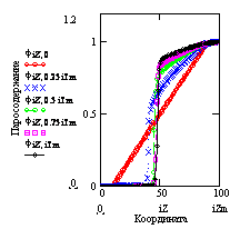
4.1. Introduction
4.2. Method rkfixed. Numerical
Instability
4.3. Method rkadapt. Integration Step
Problem
4.4. Mетод stiffr. Solution of Stiff Model Equation
4.5. Method stiffr. Solution of
Chemical Kinetics Equation
4.6. Explicit and Implicit Methods
4.7.
Conclusion
Chapter 5. Heat transfer near to the
critical point at
cross tube flow
5.1. Introduction
5.2. Integral Equation of a Thermal Boundary Layer
5.3. Mathematical Formulation of a Problem
5.4. External Flow Velocity Distribution
5.5. Deducing of Equation for the Critical Point
5.6. Reduction of the Mathematical Formulation to a
Dimensionless Form
5.7. Representation of the Right-Hand Side in the Form of an
Optimization Algorithm
5.8. Numerical Integration with the Built - In Function Odesolve
5.9. Conclusion
Chapter 6. Falkner – Skan
Equation. Hydrodynamic Friction and heat transfer in the boundary layer
6.1. Introduction
6.2. Model Construction
6.3. Reduction of Boundary-Value Problem to an Initial Problem.
Method sbval
6.4. Solution of the Initial Problem. Method rkfixed
6.5. Flow Field Imaging
6.6. Boundary Layer on the Permeable Wall
6.7. Thermal Boundary Layer Equation
6.8. Heat Transfer Law
6.9. Troubles with Odesolve -
Function
6.10. Conclusion
Chapter 7. Rayleigh’s Equation. Hydrodynamical
instability
7.1. Introduction
7.2. Hydrodynamic Equations for Free Shear Flow
7.3. Perturbation Method. Linearization
7.4. Transition in Complex Area
7.5. Numerical Integration in Complex Area. Computing Program
“Euler”
7.6. Integration and Search of Eigenvalues
7.7. Returning in the Real Area
7.8. Conclusion
Chapter 8. Kinematic waves of concentration in
ion-exchange filter
8.1. Introduction
8.2. Conservation Equation for Concentration in Filter
8.3. Wave Equation for Concentration
8.4. Dimensionless Formulation
8.5. Isotherm of Adsorption
8.6. Wave Equation Solution by Method of Characteristics (Animation 1 Animation
2)
8.7. Conclusion
Chapter 9. Kinematic shock waves
9.1. Introduction
9.2. Conservation Equation in Finite-Difference Form
9.3. Discontinuous Solutions. Shock Waves
9.4. MacCormack Method. Computing Program “McCrm”
9.5. Shock Waves of Concentration in the Filter
9.6. Shock Waves on a Motorway
9.7. Gravitational Bubble Flow. Steam-Content Shock Waves
9.8. Conclusion
Chapter 10. Numerical modelling
of the CPU-board temperature field
10.1. Introduction
10.2. Built - In Functions for Partial Differential Equations
10.3. Finite-Difference Approximation of the Thermal
Conductivity Equation
10.4. Iteration Method of Solution. Program “Plate”
10.5. Thermal Model of the CPU-Board
10.6. Conclusion
11.1. Introduction
11.2. Formulation of boundary-value problem
11.3. Discretization
11.4. Sweep Method. Computing Programs Coef
& SysTRD
11.5. Computational Modeling of Cyclical Thermal Action
11.6. Conclusion
Literature
The book include the engineering-physical projects executed in Mathcad
according to identical plan:
q
Problem-setting and physical model
formulation
q Designing of differential mathematical model,
i.e. model in the form of the differential equations (DE).
q
Numerical integration of the
differential equations
q
Visualization of results.
Uniting
attribute is the form of a nucleus of projects. In all cases it is the ordinary
(ODE) or partial (PDE) differential equations . The purpose of the book is to
help students and young engineers to design and solve the differential
equations.
Though
the projects included in the book, are educational, they contain a research
intrigue, have the important practical appendices and are not trivial in
computing aspect.
We hope,
we could find suitable combination of an engineering significance, on the one
hand, and concerning high computing complexity, with another to provide
sufficient motivation for the reference to any of modern mathematical software
packages.
Chosen
for this purpose Mathcad is the effective and rather accessible tool. Probably,
as a whole most  "democratic"
of known mathematical packages. It is especially important today when the
computer appears on working tables of the increasing number of young people.
"democratic"
of known mathematical packages. It is especially important today when the
computer appears on working tables of the increasing number of young people.
The book
consists of eleven chapters and the appendix on CD
In the
first chapter " Differential mathematical
models" the origin of the differential equations is discussed. They do not
appear at once on a working table of engineer in a ready kind for integration,
and more often should be designed by the researcher - as mathematical
models of technological processes or devices. It is not unlikely, this stage
will be the most difficult in the engineering project, and we considered useful
to give examples, how from the indistinct verbal description the differential
mathematical models of researched objects are born.
The
second chapter " Integrable differential
equations " contains the list and brief manual for the equations of the
specified type. It is shown, how to apply symbolical Mathcad processor at
mathematical calculations in this case.
The third
chapter "Dynamic model of the system with heat generating" is devoted
to systems which can develop under catastrophic scripts - with ignition and
explosion. The concept of catastrophe as some destructive phenomenon is
supplemented with a mathematical metaphor, namely, the description of dynamic
system in the form of so-called fold catastrophe from the theory of R.Toma. In this chapter are used the elements of the
qualitative theory of the differential equations.
 In the fourth
chapter " Stiff differential equations " the problem of numerical
integration of this special type of the equations is in detail considered.
Despite of practical importance of a question, it is difficult for student or
engineer to find the accessible description of this phenomenon. Mathcad has the
effective built - in function for integration of the stiff equations, but its
help system also almost nothing contains on a discussed problem. Materials of
the given chapter fill somewhat this blank. The reader will find here a plenty
of examples with use of the various integrators, discussion of features of
explicit and implicit numerical methods.
In the fourth
chapter " Stiff differential equations " the problem of numerical
integration of this special type of the equations is in detail considered.
Despite of practical importance of a question, it is difficult for student or
engineer to find the accessible description of this phenomenon. Mathcad has the
effective built - in function for integration of the stiff equations, but its
help system also almost nothing contains on a discussed problem. Materials of
the given chapter fill somewhat this blank. The reader will find here a plenty
of examples with use of the various integrators, discussion of features of
explicit and implicit numerical methods.
 The fifth chapter
" Heat transfer near to the critical point at сross tube flow " models the following situation, in which the novice engineer can
find oneself when solving of a real problem. In educational examples of
manuals the right parts of the differential equations are always set by
simple analytical expressions. In real problems the right part is
almost always represented in the form of complex algorithm, but not as
analytical expression, even difficult. Therefore, we show in action the Mathcad
structures (the programs, the built - in functions of optimization etc.) which
should be used at the decision of real problems with the differential
equations, but not only DE solvers as such.
The fifth chapter
" Heat transfer near to the critical point at сross tube flow " models the following situation, in which the novice engineer can
find oneself when solving of a real problem. In educational examples of
manuals the right parts of the differential equations are always set by
simple analytical expressions. In real problems the right part is
almost always represented in the form of complex algorithm, but not as
analytical expression, even difficult. Therefore, we show in action the Mathcad
structures (the programs, the built - in functions of optimization etc.) which
should be used at the decision of real problems with the differential
equations, but not only DE solvers as such.
 The chapter sixth « Falkner - Skan Equation.
Hydrodynamic friction and heat transfer in the boundary layer» is devoted to
numerical analysis of a fundamental problem of hydrodynamics and heat transfer.
Together with part 1.4 "«Conservation Laws" the sixth chapter forms
brief theoretical course of convective heat transfer. From the point of view of
operation in Mathcad, main theme is the numerical solution of two-point
boundary-value problem for the ordinary differential equations set with
application of built-in function permitting to reduce the boundary problem to
initial problem.
The chapter sixth « Falkner - Skan Equation.
Hydrodynamic friction and heat transfer in the boundary layer» is devoted to
numerical analysis of a fundamental problem of hydrodynamics and heat transfer.
Together with part 1.4 "«Conservation Laws" the sixth chapter forms
brief theoretical course of convective heat transfer. From the point of view of
operation in Mathcad, main theme is the numerical solution of two-point
boundary-value problem for the ordinary differential equations set with
application of built-in function permitting to reduce the boundary problem to
initial problem.
 In the chapter
seventh « Rayleigh Equation. Hydrodynamic instability
» the stability of free shear flow by a method of small perturbations
(linearization method) is parsed. The progressing perturbations, discovered at
the analysis, are the predecessors of a turbulence. In the methodical attitude,
this chapter can be the elementary introduction in stability theory. The
technique of operation with the differential equations in complex area is
considered. Is shown how to integrate the equations with complex coefficients
by the numerical method and how to interpret the complex-valued solutions.
In the chapter
seventh « Rayleigh Equation. Hydrodynamic instability
» the stability of free shear flow by a method of small perturbations
(linearization method) is parsed. The progressing perturbations, discovered at
the analysis, are the predecessors of a turbulence. In the methodical attitude,
this chapter can be the elementary introduction in stability theory. The
technique of operation with the differential equations in complex area is
considered. Is shown how to integrate the equations with complex coefficients
by the numerical method and how to interpret the complex-valued solutions.
The
eighth chapter «Kinematic waves of concentration in
ion-exchange filter» continues the theme of partial equations begun in the
first chapter by the problem about shock waves on a motorway. The physical and
mathematical model of ion-exchange filter is developed. This devices provide
with very pure water the steam plants of thermal and nuclear power stations.
The solution of partial differential equation for space-time evolution of
impurity concentration is received by characteristics method. Is shown, how the
nonlinearity of differential model results in discontinuous nonsingle-valued
solution.
 The ninth chapter
"Kinematic shock waves" continues a theme
of the wave equations.
The ninth chapter
"Kinematic shock waves" continues a theme
of the wave equations.
 The Mathcad-program
for numerical integration of the partial differential equations with effective
reproduction of shock waves is developed. Thanks to this program, research of
problems about shock waves on motorways and shock waves in filters is
completed. The problem about gravitational bubble
flows such as floating bubbles in a glass with champagne either with beer or in
two-phase contours of evaporator is in detail considered. As well as in
problems about traffic and about the filter, formation of shock waves will be
observed, but already of steam content shock waves.
The Mathcad-program
for numerical integration of the partial differential equations with effective
reproduction of shock waves is developed. Thanks to this program, research of
problems about shock waves on motorways and shock waves in filters is
completed. The problem about gravitational bubble
flows such as floating bubbles in a glass with champagne either with beer or in
two-phase contours of evaporator is in detail considered. As well as in
problems about traffic and about the filter, formation of shock waves will be
observed, but already of steam content shock waves.
 In tenth chapter «
Numerical modelling of the CPU-board temperature
field» on an example of a thermal conduction the numerical methods for partial
equations of the second order are considered. To the standard Mathcad-tools the
new program is supplemented, which permits to simulate stationary
two-dimensional temperature fields for a dilated circle of problems and to
describe correctly the thermal interaction with a surrounding .
In tenth chapter «
Numerical modelling of the CPU-board temperature
field» on an example of a thermal conduction the numerical methods for partial
equations of the second order are considered. To the standard Mathcad-tools the
new program is supplemented, which permits to simulate stationary
two-dimensional temperature fields for a dilated circle of problems and to
describe correctly the thermal interaction with a surrounding .
The eleventh chapter " Temperature waves " is devoted to
non-stationary temperature fields. Engineering appendices of this part of
thermal physics are very various. For example, in power engineering for optimum
control of starting procedure it is necessary to forecast non-stationary
temperature fields in elements of machines and the equipment, with the purpose
to exclude infringements of backlashes in moving elements because of unequal
expansion or to prevent occurrence of destroying thermal stress in massive
parts.
Interesting problem is modelling of action of
super-power energy fluxes to constructions. Almost always high-power actions
have pulsing, periodic character, and in solid bodies arise the temperature
waves. The one-dimensional non-stationary problem with interior heat generating
is surveyed as model of the circumscribed above processes and the corresponding
Mathcad-program is designed on the basis of sweep method.
Authors aspired to show on real examples how to use effectively Mathcad at
all development stage of an engineering project:
-
At analytical preprocessing the mathematical description (during normalization, research of the special points, identical transformations, etc.)
-
At analytical decisions where it is possible (or where it the opportunities of symbolical Mathcad-processor allows)
-
At the numerical decision when analytical decisions are impossible or inefficient
-
At results presentation and visualization.
We followed belief, that the basic modern tendency in engineering
researches and designing, as well as in engineering education - more and more
wide use of computer models to take into account essentially important effects
and to work with full mathematical models of objects. The engineer - researcher
should not be under pressing fears, that the developed model is too difficult
for computing and that therefore it is necessary to simplify a problem more and
more. Can be, up to such degree, that the model absolutely will cease to be
similar to real object.
At the end of the book the list of the literature is given. In addition
to direct references to sources, it includes some general literature about
numerical analysis and computer modelling, apparently,
not full. The index contains those books concerning our theme which were read
by authors, have seemed to them interesting and, hence, in the explicit or
implicit form were used during our work. From R.Hemming's
book [Ошибка! Источник ссылки не найден.] we would like
to use the following motto for our book too:
" The Purpose of calculations - not numbers, but understanding
"
Chapter 11.
Temperature waves
11.1.
Introduction
In power engineering and thermal technology for
optimum control of starting or transition procedure it is necessary to compute
the time-dependent temperature field in elements of machines and equipment.
Forecasting of a temperature field allows to avoid inadmissible temperature
rise or too big temperature drops. A characteristic example is the start
control of the powerful steam turbine on a thermal power station.
Aspiration to set in operation rapidly the
stand-by capacity, encounters the restrictions since inadmissible changes of
axial backlashes in a moving elements of the turbine because of unequal
expansion or breaking temperature stresses in massive details of a rotor and
stator turbines can arise.
More and more actual there are the problems of influence
of super-power energy fluxes on construction elements. For example, in the
problem of Controlled Thermonuclear Synthesis the heat-flux density on walls
can reach 108 W/m2.
In heavy conditions the graphite plasmatron electrodes are working. This devices are used
for high-temperature material processing. The major heat fluxes and high
temperatures arise during laser or electron-beam processing with the purpose of
surface hardening. The similar processes take place at manufacture of chips.
Almost always high-power actions have pulsing,
periodic character, and in solid bodies arise the temperature waves. The
one-dimensional non-stationary problem with interior heat generating is
surveyed as model of the circumscribed above processes (Fig. 11.1).
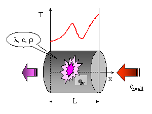
Fig. 11.1. One-dimensional non-stationary
thermal conduction problem
It is supposed, that the spatial changes happen
only along an axis of coordinates x. The lateral area is considered
adiabatically isolated. If it is necessary, the heat exchange on a lateral area
should be imitated by an negative internal heat source, is exact just as in the
previous chapter.
To provide universality of model, we shall take
advantage of the numerical method and we shall develop for this purpose the
Mathcad-program on the basis of sweep method, famous in a numerical analysis as
very-high-speed algorithm for the solution of greet system with diagonal
structure.
11.2.
Formulation
of boundary-value problem
As an initial statement we shall accept the
energy equation in general enunciation (see Chapter 1), in which the convective
transport must be eliminated and one-dimensionality,
t = t(x, τ), must be accepted. After that we shall receive:
![]()
(11.1)
At the left-hand
(x = 0) and at the right butt-end (x = L) of object (see. Fig. 11.1) there is a thermal interaction to environment, and here the suitable boundary conditions should
be set. Universal way to describe the various interactions with surroundings is
to set the boundary conditions of third kind (mixed-boundary conditions):
![]()
![]() ,
,
(11.2)
where two expressions for heat flux are
compared, namely
-
incoming from surroundings (Newton law at right hand side)
-
and conducting inwards (Fourier law at left hand side).
This equality is entirely correct only in case
of absence of phase transformation on the boundary. Generally the difference of
heat fluxes on both boundary sides will be spent for a melting, solidification,
evaporation etc. But we shall not solve here such
composite problems with phase changes.
11.3.
Discretization
To solve the partial differential equation (11.1), his finite-difference
approximation must be prepared. We receive the
necessary result, noting the energy conservation law for the small, but finite
control volume. Here it would be useful to see once again the similar
calculations which already were carried out earlier (see Chapter 1, Chapter 9).
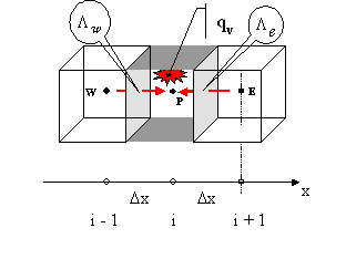
Fig. 11.2. Control volume and energy fluxes
So, we want to make up the energy balance for
control volume (Fig. 11.2), formed in a neighbourhood
of node P. The last is now in focus of our attention, but the derived further
relations will suit any interior node.
From west W and east E nodes the heat fluxes
owing to thermal conduction arrive. Inside of volume the heat source qV operates. As a result the thermal energy will
grow. And we shall detect it on rise in temperature - from T0P up to
TP in time Δτ:
![]()
(11.3)
The quantity of balance should be zero. As
capital Greek "«lambda" the relative values of thermal conductivity
are designated, which assigned to the on Fig. 11.2 specified control intersurfaces. For example, for east surface (between P and
E) :
![]() ,
,
(11.4)
were λ is the reference thermal conductivity.
Is heat conductivity constant, the single
characteristic value λ can be specified and all Λ must be as unit (1) assigned. If the thermal conductivity greatly
depends on temperature or even has disruptures
because of layer material structure , harmonic mean (11.4) ensures the heat flux evaluation
with good precision.
Equation (11.3) is given for interne nodes . Futher the similar
equation (11.7) for boundary nodes will be derived.
Implicit scheme. The temperatures in neighboring nodes, i.e. TW and TE are unknowns from "future", same as TP.
Therefore, relationship (11.3) is equation with three unknowns. The set of such equations for all nodes with
unknown temperature must be solved as system of
linear equations.
In other words: there is no explicit expression
for each unknown. Such schemes in a numerical analysis is termed implicit. They
have the important property of numerical stability, though are complicated
because of necessity to solve an equations set.
Explicit scheme. It is also possible, to attach all temperatures in the second and third
members (11.3) to "past" and to supply
they with label "0". The explicit scheme in this case is gained: each
equation contains a unique unknown value TP (in the first member of (11.3) ). The program and the evaluations
will be very simple. But if the time step will exceed some value, parasitic
oscillations will be progressing . The restrictions on a step are rather
burdensome, therefore today prefer the implicit schemes.
Detailed arguing of the explicit
and implicit schemes and the computing example are given in Chapter 1.
Let's go back to the analysis of the equation (11.3). Two variants of record further are
given. First - in the mnemonic shape, second - in index, necessary for
programming. Unknowns in these equations are temperature from
"future". The coefficients A, B, C, D are collected from known
quantities including temperature T0P, taken from the previous time
step, or from the initial conditions.
![]()
![]()
(11.5)
Comparing (11.3) and (11.5) yields the formulas for A, B, C, D.
This operations make Mathcad:

![]()
![]()
were
![]()
is Fourier-Number, the dimensionless time step.
So we receive the linear equations set with
three-diagonal matrix as shown below in the
demonstration example for the grid from five nodes :

(11.6)
The matrix of big system will appear almost
empty. For hundred nodes only three percents of meshes will be engaged, the
others will be zero. Therefore at Gaussian elimination in basic the zeros will
be handled.
However there is an express method of
elimination taking into account three-diagonal matrix structure and termed by a
"sweep" method [Ошибка! Источник
ссылки не найден., Ошибка! Источник ссылки не найден., Ошибка!
Источник ссылки не найден., Ошибка! Источник ссылки не найден., Ошибка! Источник ссылки не найден.]. Mathcad-program of this method is
given on Рис. 11.5 .
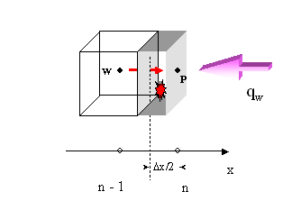
Рис. 11.3. Heat balance for a surface node
For boundary nodes, the individual expression
for the heat balance should be derived. The control volumes here appear of the
half size, as shown in Рис. 11.3. The express formulation for a heat
flux through a boundary edge should be applied (see the second member on the
right hand side) :
![]()
(11.7)
This equation is discrete analog of boundary
conditions, given above by relations (11.2). The index "inner" means
the proximate interior node: (n-1) of right butt-end, 2 - for the left-hand
butt-end. We shall not repeat evaluation for surface nodes. They are completely
similar to that are carried out for interior nodes. The final expressions can
be read in the text of the program Coef (Fig. 11.4).
11.1.
Sweep
Method. Computing Programs
Coef и SysTRD
Mathcad-program Coef
This subroutine (Fig. 11.4) compute the coefficients A, B, C, D for system like (11.6).
Vector T0 in the formal arguments list contain
the initial values of temperature. The indexing starts with unity, i.e. the
value Origin of Mathcad environment should be installed in unity. The
dimensionality of vector T0 is equal to number of mesh nodes.
Quantities Tf and Bi
are two-elements vectors specifying temperatures of
medium and Bi-numbers at the left-hand and right butt of object respectively (Fig. 11.1). The Bi- number is a dimensionless
heat-transfer coefficient: Bi = α·Δx/λ.
The parameter iTime
informs the subroutine, on what time step there is a process of calculations.
It is important for calculation of temperature of the environment contacting to
the butt. Setting in vector Pulse nonzero amplitude Ampl
and some value of frequency ν , we can simulate periodic thermal
influences.

Fig. 11.4. The subroutine for calculation of the coefficients matrix
Mathcad-program
SysTRD

Coefficients
A, B, C, D
for three-diagonal system are
prepared by subroutine Coef. In a body of procedure SYSTRD D-values will be replaced by the
calculated values of temperature. So, the procedure SYSTRD returns a vector of decisions.
Mathcad-program TimeHistory
Program TimeHistory
(Fig. 11.6) organizes calculations on time steps. The parameter nTime
sets number of time steps. Function TimeHistory
returns the temperature distributions on coordinate x for the consecutive time
moments iTime as columns of F - matrix.

Fig. 11.6. The main program
On each time step the procedure Coef is called to calculate the
coefficients A, B, C, D. Then the solver SYSTRD will be activate. With
resulting T-vector the old T0-vector of temperatures on the previous time step
will is updated and the new column to matrix F will is added.
11.2.
Computational
Modeling of Cyclical Thermal Action
The preparation of the basic data is shown on Fig. 11.7. It is supposed to investigate the
temperature fluctuations in a brass core length 39 mm when at the right
butt-end the temperature pulsing about average value 800ºC
with
amplitude 320ºC is given, and
at the left butt-end the constant zero temperature is supported.
These
boundary conditions are simulated by indicating of the requisites liquid
temperatures and such values of Bi-number which correspond to very big heat
transfer coefficients at right and left butts.
Preparatory calculations on Fig. 11.7 are clear without comments. At the
end of this fragment the T0-vector of inital
temperatures (100ºC) and also the Λ-vector of relative heat conductivity are formed.
In the given example Λ is accepted as constant. If heat
conductivity depends on coordinates and/or temperature an additional procedure
or an insert in program Coef is required. The best way of
averaging of heat conductivity will be calculation of harmonic mean values
under the formula (11.4). We leave these improvements of the program as
exercise for readers.

Fig. 11.7. Example of calculation: the basic data

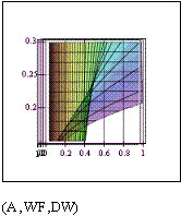
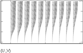
Fig. 11.8. Results of calculation: temperature waves
Results of calculations are shown on Fig. 11.8.
The right diagram represents a series of temperature distributions along
axis x
for the various time moments. More evident is three-dimensional
representation on the left diagram. The plane in the basis of the diagram is
constructed on longitudinal coordinate x
(marks 1..40) and time coordinate
(marks of time step number within the limits 1..200). On a vertical axis the
temperature is postponed. The compelled temperature fluctuations on the one of
butt-ends (mark 40 on coordinate axis) and reduction of amplitude by
approaching to opposite butt-end are clearly visible.
Showy representation of a non-stationary
temperature field can be received with the animation as it is described in
Chapter 9.
11.3.
Conclusion
We have gived only
one example of application of the here developed program. Numerical experiment
can be continued in the following directions:
q
To
investigate the influence of heat-transfer coefficient on hot butt-end temperature
q
To
investigate the influence of material properties on the maximal surface
temperature and on the heat sink through the core
q
To
investigate thr penetration of temperature waves,
having taken the long core and having set adiabatic conditions at the left
butt-end
q
To
investigate the heat transmission through the wall when the heat-transfer
coefficient on ones side will pulse in time (for that it is required to modify
slightly the program Coef, having provided the variations of
Bi-number, the same as now it was made with temperature of surrounding)
q
To
investigate the temperature modes of cylinder walls in combustion engine with
air cooling
q
To
investigate the temperature modes of building walls at weather and seasonal
changes of temperature
q
Etc.
It is possible to
analyse the majority of classical heat
conduction problems considered in educational courses, making numerical
experiment on the developed computer model. With method of computing to steady state many stationary problems can be
solved, e.g. the heat conduction in finned surface and so on. The whole complex
of educational researches may be executed for stationary and non-stationary
problems with internal sources as imitatio