If
the reader will correct translation and will send the improved text to the
author (ochkov@twt.mpei.ac.ru), the
author will tell a thank.
The story of the masterpiece
(Mathcad and nonstandard graphics)
V.Ochkov http://twt.mpei.ac.ru/ochkov (Russian
version of the article) (Another articles of V.Ochkov)
The word «masterpiece» in the title of this article should be, certainly, placed in quotes. In fact, the article title – is nothing else but the name of the TV-series presenting stories of famous canvases, kept in the Tretyakoff Gallery (Moscow – www.tretyakov.ru), in the Hermitage (St-Petersburg – www.hermitage.museum.ru), in the Russian Museum (St-Petersburg – www.rusmuseum.ru) and in other museums of Russia. Our «masterpiece» is also kept in the gallery, but this is the virtual gallery – the gallery of uncommon three-dimensional graphics enabled by Mathcad (Fig. 1).
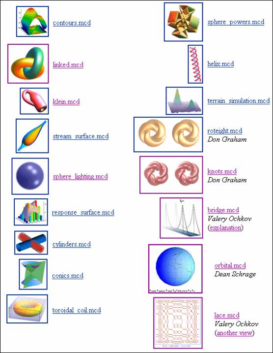
Fig. 1
The Internet address of the gallery is: http://www.mathsoft.com/mathcad/library/3Dplots. And the story of the «masterpiece» (it is displayed at the lower right of Fig. 1 and is called lace.mcd) is given below.
One of the most traditional tasks to be solved in the Mathcad environment is searching of the algebraic equation roots. Various physical, chemical and other «subject» tasks are reduced to the problem of this kind.
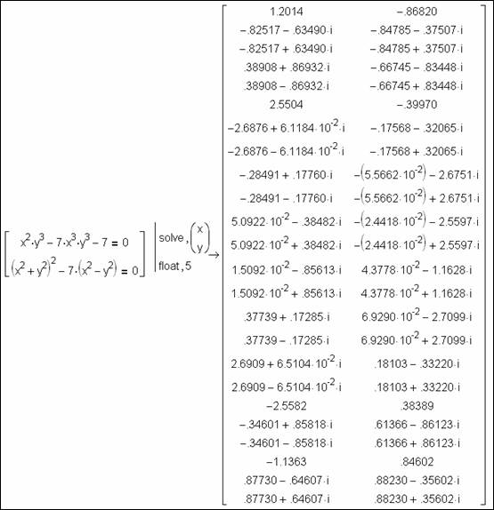
Fig. 2
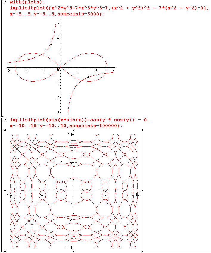
Figure 2 illustrates solution of a similar task by means of the Mathcad symbolic mathematics[1] allowing determination of all 24 roots of the set of two nonlinear algebraic equations:
(x2 + y2)2 _ 7(x2 _ y2)=0
Four of the obtained roots are real (the 1-st, the 6-th, the 19-th and the 22-nd from the top[2]), and the remaining ones – are imaginary (complex). We are lucky, so to say, with the solution displayed in Fig. 2: if any equation of the system is slightly complicated the Mathcad symbolic mathematics fails to solve the task. Operator solve, used at solution of the Fig. 2 task, – is a maximalist of a sort for it returns either all solutions of the system or none. But a user at his computer needs, as a rule, only a single real root from the range indicated by himself.
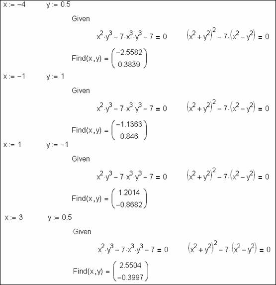
Fig. 3
Real roots of our system are searched in the example shown in Figure 3 by means of not symbolic, but calculus mathematics of Mathcad: the built-in function Find returns the values of its arguments (x and y) converting system equations (they are written under the keyword Given) into identities. More precisely the argument values returned by the function Find make deviation of the first and the second member of equations less (in absolute value) than the value of the built-in variable TOL (TOLerance, – by default it is equal to 0.001): the term «calculus mathematics» has a synonym - «approximate calculus mathematics». It is implied that symbolic (analytical) mathematics presented in the task solution in Fig.2 – is mathematics of absolutely precise calculations. Because of this fact, and also owing to that symbolic mathematics always seeks for all solutions, it appears powerless in the face of more or less complicated problem. But, we repeat it again, in most cases a user does not need absolutely all absolutely precise[3] answers (Fig. 2). He is usually satisfied with approximate values of certain roots (Fig. 3).
The God loves trinity. Complete solution of a task in the Mathcad environment should include not only symbolic[4] (Fig. 2) and not only approximate (Fig. 3) solution, but also graphical solution, which one visualizes and also verifies the solution accuracy. To solve our task graphically – means to plot two curves on the Cartesian graph, and points of intersection of these curves appear to be real roots of the system. But the trouble is that it is not always possible to reduce a system (see the foregoing example) to the form suitable for the graph construction:
y1(x) := f1(x)
y2(x) := f2(x)
Thus it is required to solve the equation f1(x, y) = 0 and f2(x, y) = 0 in x, that is rather sophisticated problem in itself and is often not solvable at all. But if an initial equation is solvable, there may be plenty of solutions – y11(x), y12(x), … y1N(x) … y21(x), … y21(x), y22(x), … y2N(x), each of them requiring for an individual curve on the diagram. We have got a certain Gordian knot, not to be untied by us: we will simply … cut it down[5].
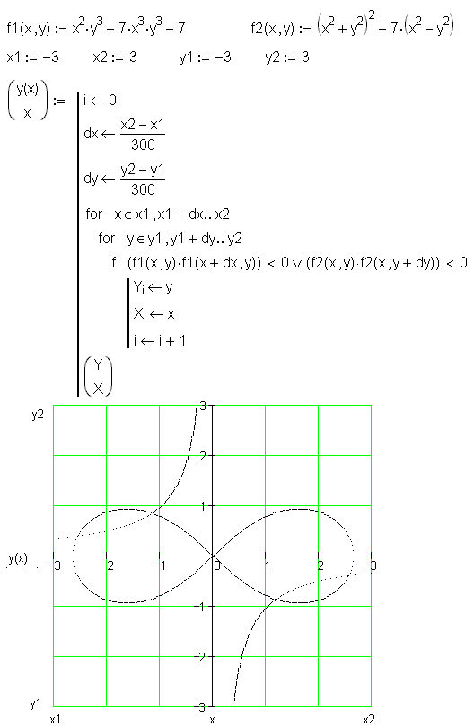
Fig. 4
Plot of the implicit function f(x,y)=0
on the MAS (Mathcad without Mathcad)
Figure 4 demonstrates a universal technique for graphical solution of the system of two algebraic equations: the surface x – y is scanned (the x and y coordinates are sorted out by two cycles for) and there are memorized the points where the function f1 or (see the operator V – the logic addition operator OR) f2 is close to zero. As our Mathcad-program is being run, two vectors y(x)[6] and x of equal depth are generated in Fig.4. The vector elements keep graphical solution of our task: intersections of curves on the graph (at the center there is plotted famous Bernoulli lemniscate[7]) – are the roots of the system under consideration. The root values are possible to be defined more precisely by addressing to Fig. 2 and Fig. 3, or by changing the values of the variables x1, x2, y1 and y2 (zooming of the graph).
And now we are getting to the above-mentioned «masterpiece» exhibited at the gallery of MathSoft, Inc. (Fig. 1).
As the reader understands, the graph construction technique presented in Fig. 4 is both suitable for a system and for a single equation of the type f (x, y). Not long ago the author (of the article and of the Gordian knot cut down technique, displayed in Fig.4) was caught with a problem «laid out» at the Collaboratory forum (see the article «Mathcad and Internet, or the Network collective farm», ComputerPress (www.compress.ru), 3’2000 – http://twt.mpei.ac.ru/ochkov/Collab/Collab.htm): a Mathcad user asked to help him to plot the graph of equation
sin(x × sin(x)) – cos(y × cos(y)) = 0.
The standard tools of Mathcad allow this problem only by means of construction of equal level curves (Contour Plot). The task solution – is the zero level line (f(x, y) = 0 – analogously to a coastline on a map). But the trouble is that it was impossible to construct a clear line f(x, y) = 0 of the above-mentioned specific equation – everything was like in a fog[8]: the curve was seen to be complicated, but what kind of curve it was, was not clear.
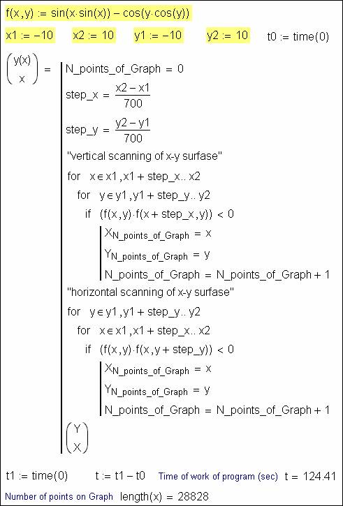
Fig. 5
Figure 5 exhibits our program of the x - y plane scanning from Fig. 4 but it is a little more complicated (duplicated): scanning is carried out not only «vertically» (for x … for y …– as in Fig. 4), but also «horizontally» (for y … for x …) in order to enhance the image sharpness, for the graph in Fig. 4 is broken into separate points at a small «rise» of the y axe.
The program in Fig. 5 inches along[9] – Fig. 6 and Fig. 7 display clear graphs of our function tatting into a lace. Our pictorial canvas is exhibited at the MathSoft, Inc gallery just by this very name (lace). We have got the square lace shawl. We pose not a Cartesian but a polar graph to be constructed by the reader to obtain a round lace napkin. Another commission – is to search for equations f (x, y) with a nonstandard graphics appearance.
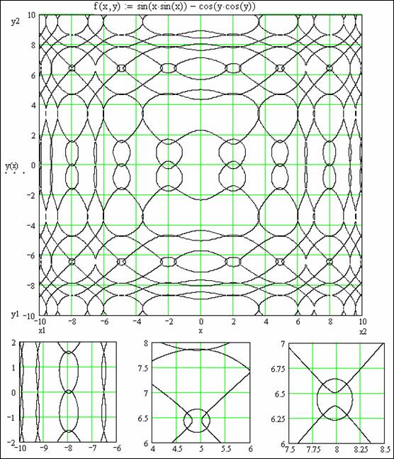
Fig. 6
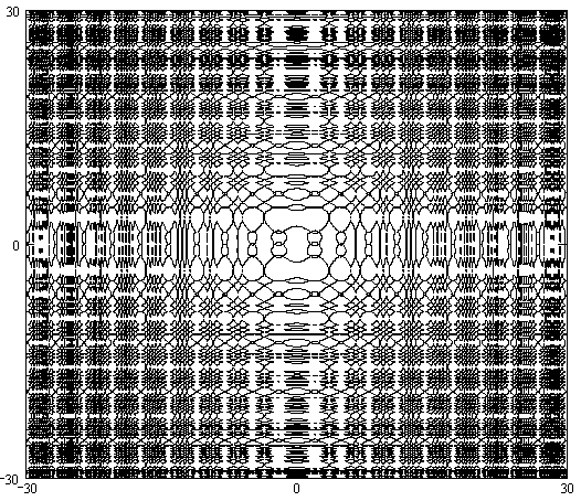
Fig. 7
In a fig.
8 it is possible to see the polar diagrams of our function, also curves
plaited in the lace – in lacy a napkin for a round table.
Fig. 1
PS
The technique of
construction of the diagrams stated above, after small completion (see program
in a fig. PS 1) suits graphic display not only
equations, but also inequalities.
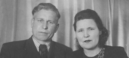
Рис. PS 1. The program
for construction of embroidery Richelieu – graphic display of an
inequality
The fine art
is impossible without colours. The author bright colours variable in the
program in a pic. PS 1:
- black – built-in constructions
- blue – User’s Variables and
Functions
- maroon – formal Variables
- green – User’s local Variables
More in detail
idea of colour in the Mathcad-programs the author has stated in a forum
Collaboratory (forum и article).
If the diagram
of function can be compared with lace, the diagram of an inequality is similar
to other sample of national creativity - on embroidery Richelieu. More
correctly, but it is less beautiful to tell, not «on embroidery», and «on a
clipping » – on a fabric do (make) "art" holes and overstitch of edge (see fig. PS 2). In
childhood of a house of the author surrounded such
napkins – them the mum covered everything, that it
is possible to cover: pillows on a bed, cases and even the TV set (КВН-49).
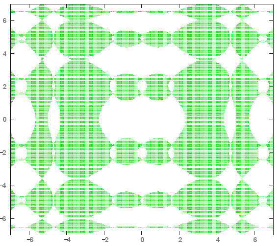
Рис. PS 2. Graphic
display of an inequality – embroidery Richelieu
The polar
display of the diagram in a fig. PS 2 is too
"beautiful" – see fig. PS 3.
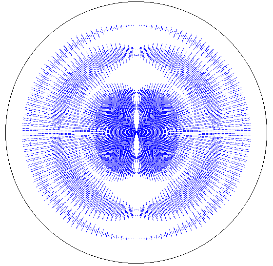
Рис. PS 3. One more
lacy a round napkin
I offer the readers «the interesting task» – search
of the equations of a kind f (x, y) = 0, on which it is
possible to construct «interesting figures».