Units in Mathcad

The questions of a solution to problems using physical values and their units in Mathcad are considered. Peculiarities of work with dimension values in computing, and symbolic mathematics in Mathcad, are also described with graphs and programs.

The second book of the series «Mathcad for Students and Engineers».

This book is aimed at a wide range of readers using computers in technical and financial calculations, as well as in the education field.

Preface for the series of books «Mathcad for Students and Engineers»

Mathcad for professionals – what does it mean?

First of all, the series of books uses an accepted template in computer literature: Windows for beginners, Mathcad for students and engineers, Excel for “kettles”, etc.

In the second place, the Mathcad-professional (in the books, you’ll often meet such «tandems»: Mathcad-document, Mathcad-operator, Mathcad-program and so on) is considered a professional in some scientific and technical range (school-teacher or lecturer, student, engineer, researcher), who becomes familiar with computers and can more or less successfully solve her or his problems with the help of a computer. But the professional does not use coding algorithms in traditional programming languages; there is not time, energy, aptitude, or corresponding inclination. And what is more one has no time for it: we all know that children become familiar with the computer very easily, compared to the problems which adults encounter. It is impossible (or rather, possible but rare) to be both an avowed luminary in some science and at the same time fluent in Visual C, Visual Basic, Delphi, etc, for creating with their help professional programs. One solution to this problem is to use demi-professional (or rather, inter-professional) programs such as Excel, Mathcad, MatLab etc.

And, finally, we have A.S. Pushkin (the first three books in the series, see titles below, were prepared during celebration of his anniversary and this is reflected in their pages). Pushkin said that he had one labour man - Pugachev. For this author, Mathcad has become a similar "labour man" - with whose help he can satisfy both his writer's itch and some financial wants. We have in mind, here, not only emoluments for articles and books, but also full and free access to the latest program releases, direct contact with the developer, and so on.

This book reflects the experience of teaching informatics and other special disciplines using Mathcad at the Moscow Power Engineering Institute (http://www.mpei.ac.ru/). One can look through the curricula of these disciplines on the following sites: http://twt.mpei.ac.ru/ochkov/Potoki.htm and http://twt.mpei.ac.ru/ochkov/Potoki_MOpt.htm..

The full series will consist of the following books:

· Advices for users of Mathcad (published – see http://twt.mpei.ac.ru/ochkov/Sovet_MC/index.htm)

· Physical values in Mathcad (this book)

· Programming in Mathcad (in print)

· Mathcad in heat engineering calculations (in print)

· Mathcad, MathConnex & VisSim (in print)

· Mathcad, DLL and ActiveX (in print)

· Graphics of Mathcad (Axum, SmartSketch and etc. – in print)

The author expresses his thanks to colleagues at MathSoft, Inc. (www.mathsoft.com) Steven Finch; Mona Zeftel, Rob Dooly and Natalia Laskaris, as well as the director of Russian firm SoftLine (www.softline.ru) Igor Borovikov, who for many years helped the author in «association» with Mathcad. The author also thanks readers of his previous books and articles about Mathcad (see http://twt.mpei.ac.ru/ochkov/work2.htm), whose comments are reflected in the present book.

Part I. Formal one

Funny story as epigraph:

Dialogue during an exam:

Teacher: What does a horsepower mean?

Student: This is the power produced by a horse with height of one-metre and weight of one kilogram.

Teacher: But where have you seen such horse?!

Student: It is not easy to see. It is preserved in Paris at the Weights and Measures Department.

Preface

Today, not only graduate students, engineers and students but also school pupils solve their tasks with a computer; but choice of Software for these purposes is problematic. We might ask: why does one more often use Mathcad for calculation of the tasks? The answer may be that Mathcad has unique features. Mathcad can operate not simply with values, but with physical values. Mathcad can be called as physico-mathematical software.

Work in Mathcad is the third (currently the highest) stage in use of computer engineering for solution of physico-mathematical, technical and educational problems. The preceding levels are work with computer codes (for example, with Assembler language) and with programming languages (BASIC, Pascal, C, fortran, etc.). These two types (computer codes and programming languages) played a spiteful joke with scientific and technical calculations. Dimensionalities of physical values, and their units (metres, kilograms, seconds and so on) were excluded. As a rule, hand solution of a physical problem (or more concrete school or student physical problem) demanded and demands use of dimensioned values. Automation of such calculations (that is composition of computer programs) excludes the «physics» of a problem. The variables of the program keep only the numerical values of variables, but the programmer has to «keep in mind» the corresponding units.

As everybody knows, human memory is imperfect. In one place one calculated the variable P, pressure, in physical atmospheres; in another place – in technical atmospheres; but in the third one – in bars. Here lies the mistake; and this mistake is based in difficulty with units bound by their values. So when we interpret a calculation into computer language it is necessary to follow a crude rule: all physical values must be in one system of units. Apart, they cannot contain factors such as 10 3, 106 and so on. This crude rule caused the following inconveniences:

The international SI system will never be universal, though it is widely used. For instance, USA uses a separate system of units similar to the British (in Mathcad this system is called U.S.). But it is the country setting the fashion in many areas of science and engineering. A program based on some one system of units prevents natural process of global exchange ideas, an even more pressing concern in the age of the Internet.
Creation of a program is divorced from its debugging. The main tool of debugging is output of intermediate results; by analyzing these we can localize and remove a mistake made when we selected formulas and/or when we wrote the program. Therefore it is important to output the physical value in the correct units of the appropriate system with the necessary factors (106, 103.and so on – see the table 3.19 in the third part of the book). Despite all advantages of the SI system, we remember that it was installed as «set of presents». Some units (kilograms, meters, and seconds) have been used without any problems, the other part. («loading») did not settle down as primary units. For instance, in heat-and-power engineering pressure of steam in a boiler is measured and expressed as atmosphere, but pressure in a capacitor is measured in millimeters of mercury. The «main» unit of pressure (the pascal, Newtons by square metre) turned out to be very inconvenient. It is difficult to think of any scientific and technical space where pascal is applied without scale factors (kilopascal, bars, megapascal and so on.). As a rule, the «settled down» unit connects with «life» (with specific physical phenomena). Atmosphere, as its name implies, is the pressure of air at sea level (approximate pressure – see fig.1.12.2 and fig.1.17.1). But, millimetres of mercury remind us of experiments by Torricelli («Torricellian vacuum», or torr; millimetre of mercury in Mathcad). In heat-and-power engineering, the exclusion of «off-system units» (atmospheres and millimeters of mercury) in favour of the pascal is not convenient. But we can get a serious breakdown in work. It is relative, for example, to the operator who controls the power-generating unit. It will not correctly interpret the display of manometers calibrated in «correct» units.
In programs we have to put in some formulas that are derived both from theoretical analysis of a problem (F=mg, E=mc2, e=mv2/2 and so on) and produced with static treatment of experimental data. As a rule, coefficients of such formulas (see, for instance, fig.1.15.1), are rigidly connected with a fixed system. These coefficients demand conversion for use in the programs, which can bring in additional error hence it will cause mistakes.

Some words about the design of the book.

This book will be published at the same time as its Internet-version (see http://twt.mpei.ac.ru/ochkov/units/index.htm). Because of the Internet version, the design of the book is special. For instance, hyper-links are displayed: see fig.1.2.1, see below, see footnote 3 and etc. Working with the book, a reader must go manually to a desired Internet page. In the Internet version, the same reader can go to new place and return more easily – with a mouse click on the hyperlink. In the Internet version, the author will make alterations and additions – he hopes that readers will send them to ochkov@twt.mpei.ac.ru.

So, we’ll return to the theme of the book.

Exclusion of units for physical values in calculations reflected on work in Mathcad. Many inexperienced users began to form Mathcad documents in this way:

they would write the dimensions of some introduced value as a commentary on, but not as a factor of, a numerical constant. The dimensions of this physical value were thus excluded from subsequent calculations. For instance, if we remember the BASIC language, the above mentioned example would contain the following form: P=20:Rem Pressure in MPa. Here, units are written as commentary (in the REM note). Using this algorithm a programmer can forget that pressure is in MPa, not in bars. Eventually, he will make a mistake.

Mathcad’s working methods with units for physical values allows:

· input of basic data in the required system, in the required units with the required factors (kilo, milli and so on);

· monitoring of dimensions in the formulas which we use in our calculation (for instance, we cannot sum kilograms and meters)[1];

· output of calculated values in required system and units, using a convenient scale for the axes of plots and so on.

One way to solve this problem is to abandon dimensional values for non-dimensional numbers that keep quantitative assessment of physical phenomenon: Re[2], Nu, and so on. When we say that the pressure in a boiler is 50 atmospheres, we operate with a non-dimensional value. We mean that the pressure is 50 times higher than atmospheric one. A more radical way is conversion from numerical to qualitative assessments - we can say that pressure is equal to some atmospheres, but we can also say that pressure is normal, high, low and so on, and form a computer-based system of control of a power-generating unit. Linguistic expert system judgements, and the theory of careless ranges, will guide this computer-based system.

In this book there are «three sources and three component parts».

Sources:

The Mathcad help system and documentation.
Basic work «Physical values» (Moscow, Energoatomizdat, 1991).
The author’s own work – articles and books that one can look through in the site http://twt.mpei.ac.ru/ochkov/work2.htm.

Component parts:

Description of Mathcad’s technology for dealing with dimension values (part 1).
The author’s collected solutions for different «dimensions» problems from literature (part 2).
Information (part 3).

So Mathcad completely supports mathematical work with dimensioned variables. Below, we’ll explain how below with the help of simple examples.

1. The simplest dimension problem

In fig. 1.1.1 the solution of the simplest physical problem in Mathcad is shown: force F has an effect on a square S, and the pressure P is to be found.

Fig. 1.1.1. Calculation of pressure in Mathcad

Physical problems in Mathcad can and must be solved with connected units for physical values. In our case it is power, square and pressure[3]. In Mathcad documents, by default, the commentary is coloured blue while mathematical expressions are black[4], namely:

Point 1.1. The variable F[5] with help of operator ":="[6] is not just assigned the number 20, but twenty-kilograms of force. The user multiplies a numerical constant by one of the system's (predetermined) variables, keeping units of physical values. In our case this variable is kgf - kilogram (kg) force (f). We can additionally print the unit using the "Master of dimensions". Its dialog window (Insert Unit) is displayed by pressing the button with an image of a measuring jug (see fig. 1.1.1). In the dialog window, Insert Unit, there are three fields and three buttons. In the first field, the user chooses the required physical value (Dimension: Force, Frequency, Inductance, Luminosity and so on), then in the second field chooses a unit (Unit: for a force Dynes, Kilogram force, Newton and Pounds force). In the Unit field, both full and abbreviated (in brackets) names are given. The third field shows the system; the user can choose and change this system. The OK button inserts the selected unit and closes the Insert Unit window. The Insert button puts in the unit and keeps window open for subsequent work. The Cancel button performs the third operation - it removes the window and does not put in the unit.
Point 1.2. Input a value of the variable S. In this case the unit is input without help of "Master dimension", since we can easily remember and insert the short form of square centimeters (cm²) from the keyboard by letters ("c", "m", "^" and "2")[7].
Point 2. Calculation of the value of pressure. Here the variable P registers both the numerical value (the result of division of the value of variable F by the value of variable S), and the result of division of the force by the square - unit of pressure.

· Point 3. Output of calculated value of pressure:

· Point 3.1. The value of division is outputted with size and dimension by default. Here the reply is added the combination of the main units of mass (kg), length (m) and time (s[8]), that are written in one line. In the expression kg × m^-1 × s^-2 we can see pressure if we at the same time multiply and divide it unit meter – kg × m / (m² × s²): combination kg_·m/s² is Newton (the unit of a force). Mathcad can not always to «guess» for the first time what dimension user wants «Some simplicity (simplification of dimension) is worse than theft+ «have stolen» meter.

· Point 3.2. The first formatting step is to write the units as a fraction but not in one line – see a tick in the Format Units field of the Result Format window in fig. 1.1.1. This window is called by a double click on the numerical result or by a command of the same name from the Format menu.

· Point 3.3. Output of the result simplified to one variable (Pa – pascal) unit of pressure. We get pascal because Mathcad (European version) defaults to SI – for international system (see the field System in the window Insert Unit in fig. 1.1.1). If we change the system – for instance we go from SI to the British or U.S. system, then pressure will be measured in an analogous «transoceanic» unit of pressure. So instead of kilograms we get pounds (lb[9]), and instead of meters we get feet (ft) [10]. Also the convention for writing of seconds changes from s to sec. At the same time, the displayed numerical value will change accordingly – it was 130755.3, and it became 87865.3.

In the example at fig. 1.1.1, scalar Mathcad variables Mathcad were available, but the user has the opportunity to unify such «single» variables into vectors and matrixes (in massifs – mathematics of the problem). Division of the dimension values by scalars and vectors is observed in physics: for instance, mass is the scalar value, but force is a vector quantity. In fig. 1.1.2 a Mathcad-illustration of Krylov’s fable «Swan, crawfish and pike» is given.

Fig. 1.1.2. Work with dimension vectors

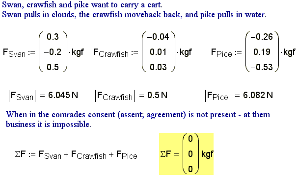
In this problem we use two tools for work with vectors (with dimension vectors). They are determination of an absolute value of a vector and vector addition[11].

Mathcad massifs (vectors and matrixes) can only hold non-dimensional values or values of the same dimension:

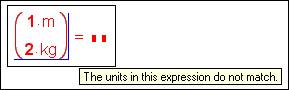
Fig. 1.1.3. Diagnostic message for error when attempting to work with a vector having elements of different dimensions

This rule has to do with computing Mathcad mathematics. To run a few steps forward (in part 9 «Symbol mathematics and units»), we must note that mathematics interprets units as simple variables. It allows us to simulate the work unit in massifs – for example, to calculate the determinant of a square «dimension» matrix:

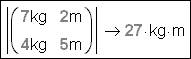
Fig. 1.1.4. Search for the determinant of a matrix, some elements of which have different dimensions

Certainly there are some situations when a result massif completed by means of computing mathematics can contain elements with different dimensions.

Fig. 1.1.5. Solution of a system of two algebraic equations with different dimensions of variables

In the fig. 1.1.5 a system of three algebraic equations with different dimensions of variable is solved. As a rule, the solution of such a problem is interrupted by a diagnostic error message, «different units». But in fig. 1.1.5 the problem was solved as we could evade two typical mistakes. Firstly, in fig. 1.1.5 data for the first approximation are zero but nevertheless they are dimensioned (x := 0 kg y := 0 m z := 0 s). Secondly, the variable where the function Find returns the obtained solution is written in а в «scalar» form and not in vector one (here a diagnostic error message appears).

In fig. 1.1.6 an attempt at a solution to the problem of a massif with differently dimensioned variables is shown.

Fig. 1.1.6. One solution to the problem of a massif with different dimensions elements

In the matrix at fig. 1.1.6, dimensioned scalar constants are divided by the base (SI) dimension. When we address the relevant matrix element, its value is multiplied by corresponding base dimension: a := M_1,1 m, for example.

2. Change of the system of built-in units

As a matter of fact units for physical values are predetermined variables, which keep a single dimension of values. Their «view» depends on the selected system – see fig. 1.2.1, where «metamorphoses» of the main three units for mass (kilogram, kg; gram, gm; and English pound, lb) are shown in three systems: SI, CGS and US.

Fig. 1.2.1. What the units for mass contain

In the fig. 1.1.1 and fig. 1.2.1, «soft» units are shown. Mathcad automatically changes them to match the user’s correction of number format (see fig. 1.1.1) or on a change of unit system (see fig. 1.2.1). But the user can put before a numerical value so-called «crude» units. They will not be changed by format (fig. 1.1.1), nor by a change of system (fig. 1.2.1). This fixation is carried out in the following way. The cursor is placed at the right hand boundary of the output operator where you find so-called placeholder (a black small square):

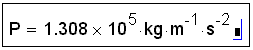
Fig. 1.2.2. «Soft» unit

In this placeholder user has the option to insert another unit. After that, «soft» units will disappear and when the user removes the cursor the new form will appear:

Fig. 1.2.3. «Crude» units

If we remove atmospheres then the old «soft» dimensioned form will come back. We can change atmospheres (atm) to other units – for example, to the main English unit of pressure (pound force by square inches – psi):

Fig. 1.2.4. Units of pressure – «crude» in SI and «soft» in U.S.

Sometimes it is worthwhile to duplicate the output operator, «typing» the reply in different units. It is very comfortable for the user to read a Mathcad-document and chooses convenient units (fig. 1.2.5).

Fig. 1.2.5. Backup of a dimension reply

Mathcad allows the previously mentioned placeholder to contain any units and any variable «visible» in a given place. If the user works in, and writes, a unit of for a different physical value, Mathcad will correct it (fig. 1.2.6).

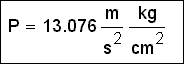
Fig. 1.2.6. Combination of «soft» and «rude» units for putting up a mistake of user

In the example shown in the fig. 1.2.6 we have tried to add a to numerical pressure value where simple kilograms (mass) were used by mistake instead of kilogram force. Mathcad has added to the «soft» unit (m/s²) to the result, and adjusted the combination of «soft» and «crude» units in as required. Finally we get the same units of pressure: force (mass is multiplied on acceleration) divided by area.

There is a similar situation when we try to add units to a non-dimensional result (fig. 1.2.7).

Fig. 1.2.7. Calculation of the number Re

In the example in fig. 1.2.7 we try to add kilograms to the number Re. Mathcad has modfied the result, writing kg^-1.

As a general rule, it is not worth changing «soft» units to «rude» ones unless it is really necessary. The point is that when you change the system of units (see fig. 1.2.1) in the document, numbers and units will automatically change.

One should remember during work with physical values that some built-in Mathcad functions return a value that depends on, so to speak, its «title» value but not on the «visible» value of the dimension argument.

Fig. 1.2.8. Rounding off a dimensioned value

In fig. 1.2.8 the work of the built-in round function is shown. This function rounds off the value of its first argument to the number of nonzero digits stated in the second argument. At first sight (point 1) one may think that the round function returns an incorrect value (a := 123.349 cm round(a, 2)= 123.349 cm, but it ought to be 123.35 cm). But if we take into account that the Mathcad-document in fig. 1.2.8 is divided into two parts with different «title» systems (SI and CGS), then everything will be clear.

Fig. 1.2.9. Construction of dimensioned range variable

In fig. 1.2.9 a typical mistake is shown. It appears during construction of a Range Variable: by default (point 1) the second element of this variable equals the value of the first element plus not one centimeter, but… one meter (the main unit of length in SI). For everything to be right it is necessary to move away from this default and say that the second element of the produced variable equals one centimeter (point 2). The zero element of the range variable can be denied the dimension; nevertheless it is better not to use this default.

Good rule. In the title of a Mathcad-document one should note to which system the document is directed. In fig. 1.2.8 and fig. 1.2.9 it is done with the assignment statement: Unit System := “SI” (“U.S.”).

The examples in the fig. 1.2.8 and fig. 1.2.9 show that it is useful to know in what system of physical values the present Mathcad-document is situated. It can be done without using menu instructions (see fig. 1.2.1), by inputting the Mathcad-document user variable created in the fig. 1.2.10.

Fig. 1.2.10. User’s variable returning the marks of the present system of physical values

3. User’s units

In Mathcad, as we have said above, Built-in-Units are introduced into a calculation either «from memory»: р := 10 kg, l := 20 mm and so on, or with help of the «Master dimension» dialogue window (see fig. 1.1.1), if user does not remember the spelling for some of the built-in units[12]. There are quite a lot of built-in units (see reference 3.4-3.17 in the third part of the book). Nevertheless in some cases user has to introduce User’s Units into a calculation. These User’s Units are connected with built-in ones by corresponding factors[13]. It is done in three cases:

User introduces into calculation a national way of writing some units: м := m, г := gm, МПа := 10⁶ Pa and so on. The first example (м := m) is trivial (m). Without any translation meters (m) will be meters for all people even they do not know any words in foreign languages. The second example is not as unnecessary as it may seem – many Russian users often get mixed up and think that the built-in constant g is gram[14], so the note г := gm (unlike the note м := m[15]) makes sense. On the other hand it is inelegant to have in our calculations a «mixture of different languages» – m (meters) and г (grams): if we are to translate into Russian units, then we must do it completely. The third example (MPa := 10⁶ Pa) we already cannot describe within the first point – It is necessary to go to point 2 and even to point 3.
The user introduces units that are absent from the built-in repertoire[16]. As an example: in Mathcad there are physical atmospheres (atm = 760 millimeters of mercury.), but no technical ones (at) – so, returning to point 1, we can write: atm := atm and atm := kgf/cm² (kilogram force per square centimeters)[17]. This way we can introduce into the calculation millimeters of water and other missing units, not just units of pressure.
The user introduces into the calculation units differing from built-in ones in degree – relating to the built-in ones through decimal coefficients. For example, in Mathcad ohms (ohm or Ω[18]), kilo-ohm (kΩ) and mega-ohm (МΩ) are built in; on the other hand there is the pascal (Ра) but no mega-pascal[19]. So we have to come back to the beginning of the calculations and write MPа:= 10⁶ Ра or, returning to point 1, МПа:= 10⁶ Ра or Па:= Ра and МПа:= 10⁶ Па. (The third point of our list has its continuation in part 4 of the book «Factors of units»).

User units input in the Mathcad-document can be grouped in the heading and added to as required. This group of operators we can isolate in the range (Area):

Fig. 1.3.1. Input of User’s units

This range, named in our case as «User’s Units», we can close (and/or protect from editing):

Fig. 1.3.2. Closed range by given User's units

But we can also remove its tracks on display and on printer papers. Another way to «hide» the inputted operators of user units is to keep them in a separate file and remark (Reference…) on it from working document[20].

User’s units can look like composite ones. For example:

Fig. 1.3.3. Input of «combined» User’s units

Division (km/hr) and multiplication (kW·hr) are not operators, but only symbols («oblique stroke», point). We can input them to a variable name by looking in advance at the mechanism of connecting of some buttons on the keyboard (symbols) with mathematical and other operators («+», «_», «*», «/», «?», «$», blank and so on). We make such an interlock using of the Ctrl + Shift + k chord (the blue cursor changes to red: «mathematics» input exchanges with input of text). For release (red cursor become blue again) we have to repeat the same chord.

For example, we can introduce into a calculation the unit of energy, the kW-hr (kilowatt -hour). Here the symbol «minus» is not subtraction, it is multiplication: kW-hr := kW·hr. This example, «Do not believe your eyes!» series, prompts us that in calculations it possible and necessary to input units which are accepted in text or verbal descriptions of physical values[21].

Input of user units within calculations is not ideal. We have to try to manage with those units that are built-in to Mathcad. This is because when transferring some fragment of one Mathcad-document to another one we can «lose» the user’s units formatting. It will be fraught with errors such as «The variable is not definite». Besides, user’s units are «crude» units, so they do not change when we change the system (see fig. 1.2.1). User units are a good and useful thing when a client gets the calculation not as a Mathcad-file but as the printed calculation containing exactly those units in which the client is accustomed to working.

4. Factors of units

In point 3 of our list we have previously shown how we can introduce into our calculations new (user’s) units, connecting them with built-in ones with the help of coefficients divisible by ten: MPa := 10⁶·Ра, MW := 10⁶·W and so on. In this way we eliminate some «discrimination» relative to separate built-in units. But we can do it in another way: by introducing into a calculation user's factors of units but not user’s units[22]:

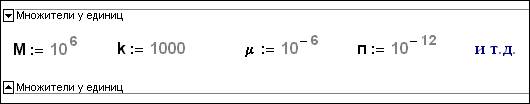
Fig. 1.4.1. User's factors of units

New units are introduced into the calculation by multiplying a user's factor on the main built-in unit:

Fig. 1.4.2. Work with User's factors of units

«And etc.» in the given list one ought to read as: «see the table 3.19 in the third part of the book», where all possible factors in calculations are showed. If in our examples we change the sign of multiplication (·) to «no space» (No Space is possible in Mathcad 2000), then the illusion of united units rather than complex ones will be complete:

Fig. 1.4.3. Input factors of units

However, there is one problem. Some factors and some units are written in the same way: m is a unit meter and milli (10^-3), с is both a second (in the written Russian form) and centi[23], etc. In this case one can understand the note mm both as millimeter (10^-3 m) and as … square meter (m² = m·m or m² = mm). We must remember that the absence of some symbol between two variables in Mathcad (and not only in Mathcad) can mean multiplication. Reading the note mm as rule we intuitively put in between two letters m the sign of multiplication and consider that it is different value: the first one m is 10^-3, but the second m one is the unit meter[24]. In Mathcad this misunderstanding is solved in contrast to common programming languages – see the part 8 of the book «Styles of variables and units».

5. Units with suffix (mass or weight)

Many inexperienced users of Mathcad encounter the problem in the title (mass or weight). The developers themselves bring into the Mathcad package a degree of mishmash. So, in the part devoted to Pressure in «Master dimensions» (Insert Unit… see fig. 1.1.1), the unit psi is decoded as Pound per Square Inch. At that time in reality a unit of mass (lb/in²) does not figure there, but unit of force (lbf/in² – pound-force per square inch). Outside the effective area of the British measure system (S.U.), users make similar mistakes. For example, they introduce technical atmospheres into calculations as аt := kg/cm², where it should be аt := kgf/cm² and so on. In the previously mentioned examples, two main built-in units of mass, kg (SI) and lb (U.S.), are involved and two additional built-in units of force (weight) kgf and lbf.

We can say weight as a dimension «hangs» between force and mass. By its physical essence – it is force. But by its name of units – it is near to mass: kilogram, pound (in brackets one usually shows that it is not simple kilogram or pound but it is kilogram-force (pound-force); but often one forgets about it, assuming that people will automatically understand). Also, the common way to measure a body’s mass is weighing on scales. Once more we get some mishmash between the notions of «mass and weight»[25]. In one Mathcad-document with important calculations, this author has seen the determination кг: = kgf. Here the notions of mass and weight (force) are confused. The author of that document explained it as follows: he said that in his field of knowledge kg was and would be a unit of weight, not a unit of a body’s mass. If we calculate according to demands of SI, then it is necessary to write all textbooks with the given discipline. In this case it is difficult to judge where the fault lies, but the trouble originates with the specialist who laid the foundations of this science. But the operator kg: = kgf in the calculation «is like a time bomb that is ready to blow up in any moment» – it is easy to forget that kg is not mass but it is a force.

Only two «privileged» built-in units kgf and lbf have the suffix «f» in Mathcad. But it (the suffix f) can be added to other units of mass. The first way is through introduction of user’s units of force (gram-force) gmf := 10^-3 kgf, (ton-force) tonf := 10³ kgf etc into a calculation. The second way is shown in the fig. 1.5.1, with the constant f introduced into a calculation. It (the constant f) is a dimension factor (speeding-up) connecting mass and force (weight): kg = f kgf (Newton’s second law).

Fig. 1.5.1. Suffix of units

Now for units of mass to be turned into units of force it is enough to multiply unit of mass on the constant f. As the reader already knows, in Mathcad 2000 the sign of multiplication can be removed, combining the factors: kg f → kgf. So we get the full illusion of unit of force[26].

Commentary. We can introduce into a calculation the coefficient m (m := g^-1) for transfer units of force to units of mass: Nm (Newton of mass), dynem (dyne of mass) and etc. But in this way we may confuse all Mathcad users: m is the meter unit, m is the factor 0.001 (this «mishmash» we have already mentioned above, inherent in the foundations of SI), m is the suffix for transfer unit of force to unit of mass.

6. «Non-dimensional» units

One such «non-dimensional» unit has already been built into Mathcad. It is percent: % = 0.01. Actually it is not a unit but a simple factor (fig. 1.6.1).

Fig. 1.6.1. Percents in Mathcad-document

We can introduce other similar pseudo-units into calculations – (thousandth – ‰:=10^-3), for example. We can introduce into calculations units of concentration (fraction): fraction of total mass, fraction of total volume, mole (molar) fraction etc. To «service» them we can introduce into calculations additional user’s «non-dimensional» units:

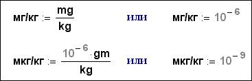
Fig. 1.6.2. «Nominal» factors in Mathcad-document

In English-language literature these units of concentration are denoted as ppm (part per million – millionth fraction, mg/kg) and ppb (part per billion – billionth fraction, mkg/kg[27]). But designation with the help of mass units (mg/kg), volume (ml/l) or agent quantities (mmole/mole) are «more clear», than ppm or ppb are. There we can see what fraction (part) we are talking about: fraction of total mass, fraction of total volume or molar (mole) fraction. For example, in chemistry SI allows us to measure concentration of calcium in water only in mmole/kg. But in practice one continues to use such «unlawful» units as mgг-mole, mg-eqv/kg, noting that in solution we can calculate either ions (mg-mole), or charge of calcium ions (mg-eqv), there are two on every ion.

It is useful to introduce into a calculation units equal to unity[28]. Fraction (of total mass, of total volume or molar one) can be measured in such units as: kg/kg, ml/ml and mole/mole, but it is nothing else as simple unit, that is squared unit: mg/mg = 1.

Often in calculations we meet things by way of units of agent quantity:
thing := 1 Weight := 5 kg/th Quantity := 10 Common weight := Weight quantity Common weight = 50 kg.
Sometimes we have to use other counting units in our calculations – pairs, tens, dozens and so on[29]. Sometimes these units are attached to concrete examples: pair of shoes costs seven hundred rubles, ten eggs cost twenty rubles and so on. (About rubles you can see below in part 7 «New dimension»). Such appraisals do not differ, for example, from the notion of specific gravity, when we divide weight on volume. Pair of shoes and ten eggs are units of two physical values that we can not add up – just as we cannot add up kilograms and meters[30].

Counting units get into SI as moles. In a practical manner we can not use them for fixing «worldly» structural units: things, pairs, dozens. The mole is 6.022×10²³ things of structural units. A mole is the number of molecules in 12 g of carbon–12. Moles do not satisfy even chemists completely. They have to introduce the additional units of agent. Or rather they have to introduce the additional dimension in a solution. For example, as we have said above moles (g–mole, mg-mole[31]) measure number of atoms, but number of ions is measured by equivalents (g–eqv, mg-eqv). We can consider that moles of oxygen, for example, and moles of hydrogen are units of different physical values. They are different because we cannot add them (as with pair of boots and ten eggs, since we get «soft-boiled boots»). We cannot do it as long as we regard as the compound reaction of two atoms of hydrogen with one atom of oxygen. Why does SI have exactly seven dimensions? An echo of metaphysics is heard in this system of physical values. There are seven dimensions in SI because … there are seven colors in rainbow; there are seven notes in octave etc.

The decibel (dB) is an original «non-dimension» unit. The bel is the decimal logarithm of ratio of two of the same name physical values[32], but decibel is accordingly one-tenth of a bel. Measuring something in decibels we form in this way some scale (sliding-scale) of values of physical values. In this we have to choose some base from which we commence counting. In fig. 1.6.3 such a scale is formed relative to power. The power of a human’s heart[33] is taken as the base:

Fig. 1.6.3. Work with decibels

For work with decibels, two functions with names dB (the name of one function is invisible – we write in white on white[34]) and one constant with the same name dB are input in the Mathcad-document. But they are different objects as they have different styles. As marked in the footnote, an «Invisible» function serves for output of the value of the dimension variable in decibels, but the «visible» one for input. It is called not in traditional form but as a suffixed operator: not p := dB(100), but p := 100 dB. In this way a unit is simulated (continuing the theme of using not factors but operators during work with units in part 14 «Relative scales»).

Commentary. Mathcad sometimes shows excessive pedantry during output of dimension values. So if in Mathcad we type kg – 1000 gm =, then we get reply 0 kg, although it is enough to have one zero without more precise of units: zero mass is zero one in any units of mass[35]. In such a «calculation» situation it is worth changing the style of zero-output units to «invisible» (in white and white). It is done in fig. 1.6.3, when we output zero power of infinity decibels.

Fig. 1.6.5. The problem of rpm

7. New dimension

One can argue about whether cost (price) is a new dimension value or not. Physiatrics may easily say: «On my table there is a book of one kilogram weight, three centimeters thickness and cost 1000 rubles. But the same physiatrics consider as absurd and even seditious the idea that cost enjoys the same full rights of dimension value as weight or length (thickness). These disputes continue and they will not finish soon. This is reflected in Mathcad, which does not have such value as cost. However, we’ll not argue about it but we show how in Mathcad we can link units of cost to introduce corresponding dimension values, for checking dimensions and outputting dimension values.

We can introduce a unit of cost into calculations with some built-in value not used in the given calculation, for example luminous intensity[36].

Fig. 1.7.1. Work with economic value

In fig. 1.7.1 one keeps an account of payment for electric power – they worked 150 days on a power of 300 watts. Unit of cost temporarily is equaled to candela: rouble = cd – see point 1 in the fig. 1.7.1. The result (payment for electric power – see the point 4) will be given in candelas[37] («soft» units), which we must return in roubles[38] («crude» units) – see the last line in the fig. 1.7.1. We can in the Mathcad-document at fig. 1.7.1 write ruble := 1 but not ruble := cd. But if we connect units of some new value with some built-in one that are not used in the given calculation, it allows us to keep the control of dimensions[39] mechanism. The point is that the input into the calculation units allows both the response in scale physical values necessary for the user (in one case it is better to get pressure in atmospheres, but in another case - in millimeters of mercury etc) and to block up the addition of meters with kilograms.

In fig. 1.7.2 one approach to the solution of these problem is shown. This was a live problem at the time when this book was being written and apparently it will be continue to be so for a long time – until supplies of mineral oil run low. In the middle of 2000 the price of mineral oil increased with impact upon the cost[40] of petrol. Producers of mineral oil and consumers of oils (for example drivers as a token of protest blocked up roads of Europe and USA) saw different ways to solve this problem. One considered that it was necessary to cut taxes that increased the price of petrol. The other called for an increase mineral oil quotas to decrease its price. But the main thing that we can see in fig. 1.7.2 is the mechanism for working with dimension values of cost (price) and volume.

Fig. 1.7.2. Appraisal of the structure petrol’s price

In fig. 1.7.2 the barrel is introduced as a user’s unit of measure of volume with the help of the gallon but not the litre (bbl := 0.158988 L). Firstly this definition is more accurate, secondly it is easier to remember.

The operator rouble := cd does not serve for work with financial functions that are introduced in Mathcad 2000. These functions can work only with non-dimension variables. That’s why on calling them it is necessary to deprive the variables their dimensions (see solution 1 in fig. 1.7.3). The other way that we have already described – in Mathcad-document units of measure of cost are worth to input following way: RR := 1 $US := 28 RR and etc. (see the solution 2 in the fig. 1.7.3). But we have to remember the possible mistake of summing roubles with non-dimension values.

Fig. 1.7.3. Work with financial function of Mathcad

The examples of calculations with user’s units of cost (price) are shown in part 9 «Symbol mathematics and units» in the second part of the book.

8. Styles of variables and units of measure

Mathcad has the unique ability to operate in calculations with the same name and the same format[41] variables. Nevertheless these variables are different because they have different styles. Such variables «live independently», and they do not get mixed up with each other.

This feature of Mathcad is suitable in working with units.

By default style Variable, Constants[42] are assumed to be variables and functions introducing into calculation:

Fig. 1.8.1. Built-in styles

The style Variable is attached to variables that from the beginning are «charged» with holding units which user introduces[43] into calculation. Because of this, contradictions can arise in the calculation: for example we have measured sides of rectangle and want to calculate its square:

Fig. 1.8.2. Calculation of the square without using styles

In this example we deliberately exaggerate the mistake with which users of Mathcad are quite often in conflict. This mistake is related to involuntary or intentional (as we have in our example) overdetermination of built-in variable. Certainly users will hardly give the names hectare and acre[44] to the variables keeping sides of rectangle. But if sides are named m, for example, or L, then here we mistake easily arises: m is meter, but L is litre. If with variables hectare and acre the same name but different by sense are assumed different in style, our program (see above) will work well enough – sides of the rectangle are fixed to the user’s style[45] with the name User 1, but the units have built-in style Variables:

Fig. 1.8.3. Calculation of the square using the styles

Division of the variables will help us to solve the contadiction mentioned above in part 3, «mm»:

Fig. 1.8.4. Division of styles of variables

In the example in fig. 1.8.4 there is not only one object with the name mm, but there are three: mm are millimeters, mm are squared meters and mm is the factor 10^-6. Such «variant reading» appeared because in the calculation there is not only one, but there are two variables m with different styles. So that we do not entangle in the calculation, it is worth giving different color, type or size of the type to different variables. For example, the author practices the following approach to picking up units of measure in calculations. He practices and recommends this to his students: variables keeping units of measure are assumed the style with the name Unit and brown color, so that we can pick up these variables in calculation. (Commentary. Sometimes it is necessary to have the same names, but different style variables and functions, connected with units of measure – see part 14 «Relative scale of measure»).

9. Symbolic mathematics and units of measure

If computation mathematics in Mathcad operates with numerical values kept in variables, symbolic mathematics operates with variables. It allows rather simply solving problems with the same dimension that are not native to Mathcad.

In fig. 1.9.1, with the help of Mathcad’s symbolic mathematics, the problem from Chetov’s story «the Coach» is solved: «A merchant bought 138 arshine of black and blue cloth per 540 rubles. It is asked, how many arshine he bought of black cloth and how many arshine he bought of blue cloth if blue cloth cost 5 rubles per one arshine, but black one cost 3 rubles per one arshine.»

Fig. 1.9.1. The problem on the merchant and the cloth

In the solution of this problem, units of measure are simple variables. One can apply computer analytic conversions to them to determines a «dimension» response: the merchant bought 63 arshine of blue cloth and 75 arshine of black.[46].

Mathcad users who «enjoy the charms» of dimension values in numerical calculations automatically transfer their experiences of work with meters, kilograms, and seconds to symbolic mathematics. But they forget that analytic conversions to units of measure do not work. We mean that in Mathcad[47] symbolic mathematics «does not know», that there are a hundred centimeters in one meter, but ohm is volt divided by ampere and so on. That is why it is necessary to lead analytic conversions with collaboration of different units of measure. So it is necessary to prompt to symbolic correlations between them.

Fig. 1.9.2. The solution of dimension problem with help of symbol mathematics

Fig. 1.9.2. The solution of dimension problems using symbolic mathematics

In fig. 1.9.2 the simple equation I + v/r = g is solved for the variable g, the variables v, г and I being dimensioned (voltage, resistance and current strength). We only obtain the correct solution using symbolic conversion when we include in our conversion Ohm's law[48]: to exchange ohms with volts divided by amperes.

Fig. 1.9.3. Finding a determinant of a matrix whose elements, which have different dimensions, are expressed in different units

In fig. 1.9.3 the solution to the problem of a search for the matrix’s determinant is shown. The matrix has dimensioned elements (fig. 1.1.4). Furthermore, equidimensional values are given with different units of measure. The right solution of the problem, as in the example in fig. 1.9.2, is possible only then if we point out the correlations between units of measure.

Solving dimension problems with the help of symbolic mathematics we have to remember that there is no control of dimensioned values in Mathcad’s analytical conversion – see fig. 1.9.4.

Fig. 1.9.4. Numerical and analytical output operators: control of dimensions

10. Physical values without units of measure

Few people remember now that in early version of Mathcad (for example, in DOS-version[49]) there were no built-in units but three built-in variables (1T, 1L and 1M). Length, Time and Mass were attached to these variables. So, if it was necessary to introduce concrete units of measure into calculations, one acted as follows:

Fig. 1.10.1. Dimension in DOS-version of Mathcad

It is possible not to introduce units of physical measure but to work with abstract dimensions.

As we can see from fig. 1.10.1. the system of measure was «stitched» in DOS-version of Mathcad. This system was based only on three values: length, time and mass (the MKS – meter-kilogram-second or CGS – centimeter-gram-second – system). Then in new versions of Mathcad charge (or current strength), temperature, quantity of agent, luminous intensity and …appeared. Now, L is not a physical value named «length» but a unit of volume named «litre», Т is not time, it is tesla (unit of inductance[50]). The names of some dimensions have become the names of built-in functions: length –already the name of the function returning the vector’s length, time – an undocumented built-in function, fixing the work time of the computer[51] and so on. The «triple» system of physical values (time – length – mass) from one to another version of Mathcad grew into a «septenary» one (SI) that defined some mishmash in the designations of units. But the Mathcad user has the right to refuse concrete units of measure and work with abstract dimensions based on designations accepted in SI.

For this there are two possibilities – they are built-in and user’s ones.

First of all, using the Dimensions label in the Math Options dialogue box, called by the Options… command from the Math menu, it is possible to turn off the output of units of measure by changing their names to the corresponding names of physical values (fig. 1.10.2).

Fig. 1.10.2. Change of units of measure to physical values

Built-in the (English) names of physical values it is possible to change into user’s ones – into Russian, for example:

Fig. 1.10.3. Work with user’s names of physical values

Alternatively, it is possible to introduce into calculation seven variables that denoted the main seven physical values (see fig. 1.10.4 and the table 3.4 in the third part of the book):

Fig. 1.10.4. Work with dimensions but not with units of measure

Depending on generally accepted designation of the main dimension values it is possible to fill in the Dimensions bookmark of the Math Options… dialogue window (see fig. 1.10.5):

Fig. 1.10.5. «International» contents of the bookmark Dimensions of the dialogue window Math Options…

11. Control of dimension

As we can see from fig. 1.1.1, given in the beginning of the book, the technology of the Mathcad solution exactly repeats the technology of the «handmade» solution: input data are introduced (point 1 in the fig. 1.1.1), calculation takes place and finally the result is output. In this case the creator of the Mathcad-document has the right to demand from future users the input of both initial values of variables (number) and the necessary dimensions.

Fig. 1.11.1. Control of a dimension of a variable

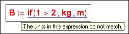
In the fig. 1.11.1 one way to control dimension is shown[52]: the unit meter is added and at the same time is subtracted from the input variable. The input variable does not make any changes. But if this variable is non-dimensional (or has some dimension but this dimension is not length but some other value) then the calculation is interrupted by the error message: «The units in the expression do not match» and «This variable or function is not defined above». The operator d := d + m - m is a little strange from the traditional programming point of view[53], but in Mathcad this operator is regular enough if we remember that m is the meter unit. Besides, in Mathcad one can have the same names for different variables denoted as Variables and User1 (see part 8, «Styles of variables and units of measure»). We use it for dimensional control of the variable d.

For dimension control of some variables it is possible to use the built-in function UnitsOf, returning unit of measure of its argument – fig. 1.11.2.

Fig. 1.11.2. Work of the function UnitsOf

Actually the function UnitsOf returns not units of measure but the dimensions of its argument. That’s why this function should be renamed as DimensionsOf. Fig. 1.11.3 shows its operation during included conditions. This function reflects direct dimensions but not units of measure (see fig. 1.10.2 and fig. 1.10.3).

Fig. 1.11.3. Output of names of dimension values

(The dimension control theme is continued in the part 13 «Dimension in programs» – see fig. 1.13.1).

12. Dimension on graphs

It is possible and necessary to use units of measure of physical values in both calculations and graph design.

Fig. 1.12.1. «Dimension» graph

In fig. 1.12.1, the behaviour of atmospheric pressure by altitude above sea level using barometric formula[54] is shown. The results of the calculation are output as graphs – the left graph is for continental Europe, the right graph is for USA and Great Britain. If we denote the axes thus: the ordinate axis as p (h), but the abscissae axis as h (altitude that we discretely change (tabulate) from 0 to 20 km with pitch 100 m), then the scales of axes will be graduated in pascal and in metres. These are the main units of measure of pressure and length (in our case it is altitude) in the system SI. If we change the system of measure from SI to U.S. (see fig. 1.2.1), then the graduation of axes will change to psi (pound force per square inch) and ft (feet). But in fig. 1.12.1 we have drawn both graphs with subsidiary units. The change of axis graduation in the necessary direction is done as follows: user changes the note p (h) to p (h)/necessary unit of pressure and h to h/necessary unit of length. In this way we choose required graduation of axes of the graph – metrical, British or some other: meters instead of kilometers, milli feet instead of hundred feet, mm (inches) millimeter of mercury[55], atmospheres and so on. So we build the graph to optimal human perception. In fig. 1.12.1 the names of units of measure on the axes are written by commentaries which repeat the names of units in denominators of expressions near the axes.

We should remember that when we construct the graphs, the dimension control mechanism turns off. This peculiarity is illustrated by the Mathcad-document in fig. 1.12.2. Here the following problem is solved: it is necessary to construct a dependence of the volume of liquid residue in a tank (V) from maximum depth of liquid[56] h.

Fig. 1.12.2. Graphing the behaviour of liquid volume residue in a tank

The peculiarity of the Mathcad-document in fig. 1.12.2 is that the user does not assume anything of the variables L and R, but nevertheless the graph is created. The point is that that the variables L and R are defined by the system (see fig. 1.12.3).

Fig. 1.12.3. What do the variables L and R hold?

L – is litre (volume), but R – is Renkin degree (temperature). But when we construct the graph in the fig. 1.12.1 we temporarily consider that these variables are non-dimensional: L := 10^-3, but R := 0.5(5).

The property of Mathcad not taken into account by dimension of values when constructing graphs will help us to solve next problem-joke: «Who is greater (more famous), Gauss or Newton?» The solution is in the fig. 1.12.4.

Fig. 1.12.4. Gauss or Newton

Certainly it is possible to compare neither Gauss with Newton nor gauss (unit of magnetic flux) with newton (unit of force). But the graph in Mathcad (see fig. 1.12.4) shows that newton is greater than gauss.

13. Dimension in programs

Programming in Mathcad has three attributes:

1. Local variables.

2. Unification of separate operators to programming blocks, that are in progress as united operators.

3. Change of order of fulfilment of operators (cycles or alternatives).

There are no special problems with two first attributes of programming before units of measure. In fig. 1.13.1 the formed function V (D, L) is shown. This function is formed with the help of programming tools and the function returns the volume of a cone (V) depending on base diameter (D) and length of generatrix (L).

Fig. 1.13.1. Programming the calculation for volume of a cone

In fig. 1.13.1 three examples of the function call V (D, L) are shown. Two of them are unsuccessful (or rather, they successfully cut off attempts to input wrong data: arguments are non-dimension or have wrong dimension) resulting in output of the built-in diagnostic error message, and only one is successful (arguments have the right dimension – length). The control of dimensions of arguments (as in the example in fig. 1.11.1) is led by addition the + m - m, omitted in the first and in the second cases where the user (by mistake or on purpose) inputs the argument values without units of measure or with wrong dimension. In fig. 1.13.1 the values of formal variables D (its half) and L is carried in local variables R and L by the first two operators of the program. The values of the variables D and L are the same (we add and at the same time subtract from them the unit meter). But if the user of the function inputs arguments with wrong dimension or without dimension, then the diagnostic error message «inadequate in units of measure» will interrupt the execution of the program[57].

As we can see from fig. 1.13.1, units of measure built-in to Mathcad do not have any problems with the first two attributes of programming – with local variables and program blocks. The conflict appears when programming changes in the order of fulfilment of operators (the third attribute of programming) – when using the structural manager structures: cycle, alternatives, as we can see from the fig. 1.13.2.

Fig. 1.13.2. Dimension values in the shoulders of alternative

In the documentation of Mathcad there are no words about using units of measure of physical values in programs, but in «Day advices[58]» one can read: «In the programming language of Mathcad following of units of measure within cycle is not lead. That is why it is not worth assuming units of measure to variables, use within program». But this method of using units of measure in programs is very alluring. It is necessary to remember the following limitations:

1. As we have mentioned above, the mechanism of dimension values can cause some bugs when we use structural manager operators – if, for example. It touches both the programs with the operator if, and «without program» Mathcad-documents with the if function. So the operator

gives the bug – arguments of the function if (shoulders of alternative) can only be non-dimensional or of the same dimension.

2. Very often in programs we have to group local variables to massifs (to vectors or matrixes). It can prevent the use of units of measure: massifs can hold only non-dimensional values or values of the same dimension.

3. Many built-in Mathcad functions can only have as arguments non-dimensional values and/or values of the same dimension. The same peculiarity touches on massifs that returned the built-in functions.

Previously mentioned points allow us to give the following advice about using dimension values in programs: it is necessary to deny in the program values passing their dimensions by the first operators of the program. But with the help of the last operators it is necessary «to print in addition» the necessary dimension to the returned value.

Fig. 1.13.3. Work with units in the program during debugging

In fig. 1.13.3 the model of the program is shown. This program is created subject to previously mentioned advice: the user’s function for calculation of the volume of the cone is formed (fig. 1.13.1). For the input lines of the program we do not use the operator Add Line, but… the matrices 2 per 5. The elements of the matrix are either commentaries (the first column), or the operators of the program. The program works without bugs during the debugging operation, when all local variables are output on display, and during «work operation», when only the volume of the cone with elected unit of volume[59] is returned.

The above-stated limitations on use of units of measure in programming affect Mathcad 2000 Pro[60] and earlier versions. During the time when author has been writing this book, Mathcad 2001 Pro has appeared, where many defects are corrected – see fig. 1.13.4 and fig. 1.13.5.

Fig. 1.13.4. Work of the operator return with dimension operand

In Mathcad programs there were problems with using the return operator during return of dimensioned variables (see fig. 1.13.4). Primarily (Mathcad 2000 Pro and below) the return operator returned the correct numerical value but the wrong dimension (the dimension of the last variable in the list of the return operator). Then (in «patch» С) this mistake was touched up, but it not adequately – the return function began to return non-dimension values of any values of its operand. In Mathcad 2001 Pro this mistake is addressed. The mistake arising from use of dimensioned values in the function and operator if (see fig. 1.13.5) is also dealt with.

Fig. 1.13.5. The function if and the operator if in Mathcad 2001 Pro

Though many mistakes, connecting with dimensions in programs, are corrected in the new version of Mathcad, the author has considered it necessary to place in his book some peculiarities of work with dimension values in programs under different versions of Mathcad.

The mistake concerning orientation to default units of measure (see fig. 1.2.8 and fig. 1.2.9) can appear in programs when by default the second value of the variable of the cycle with parameter is not given.

Fig. 1.13.6. Default reducing to a mistake in the cycle with parameter

This mistake is shown in fig. 1.13.6. If in the title of the cycle one writes L Î 1 cm. 7 cm, then the Mathcad system, directed to SI where the main unit of length is meter and not centimeter, considers that the second value of the cycle’s parameter must equal … 2 meters. To eliminate this mistake it is possible either to change the system of measure, or by giving default increase when forming the title of the cycle for: L Î 1 cm, 2 cm. 7 cm.

14. Relative scales of measure

In the list of built-in units for temperature there is Kelvin, (K) and degree Rankin (R)[61], but not the degree Celsius or Fahrenheit degree[62], both widely used in engineering calculations. The point is that there are two metrical notions to this physical value – unit of measure of temperature and scale of measure of temperature[63]: degree Celsius equals Kelvin, but scale Celsius is moved relative to Kelvin scale by 273.15 degrees (Celsius or Kelvin[64]). Because of it we cannot apply the simple rule of creating user units (scales) of temperature by connection with built – in suitable factors (see part 3 «User’s units of measure»).

If the user of Mathcad wants to introduce into calculation values of temperature orientated to Kelvin or Celsius scales, he can do it in this way as follows from the fig. 1.14.1.

Fig. 1.14.1. Input of temperature about relative scale

But this solution (we have, by the way, already used this solution in the Mathcad-document in fig. 1.12.1) cannot be considered a complete one – it is desirable both to input (without subsidiary addition operator) and to output temperature values in degrees and by scale Celsius (or Fahrenheit).

In fig. 1.14.2 we show one of the solutions to this problem. We try to do it on a simple example: two temperatures are given, and we have to find a difference between them. It is clear that this is not an arithmetic problem, but a metrological one. All values have the dimensionality of temperature. The users can input and output the value of temperature in any one of four units of measures and scales: Kelvin degrees (scale), Rankin, Celsius and Fahrenheit. For this we introduce into the calculation eight objects with the names °C and °F:

· two functions with the name °C[65] (the first one °C(t) := (t+273.15) K style – Variables, and the second °C(t) := (T/K-273.15) – Units 1, with color of the name of the second function being white. It is invisible on the display screen[66];

· two constants with the name °C (the first one °C := 1 style – Units 2, and the second °C := K – Units 3);

· two function with the name °F (first one °F(t) := (t+459.67) R style – Variables, but the second °F(T) := (T-459.67) – Units 1, with color of the name of the second function being white. It is invisible on the display screen;

· two constants with name °F (the first one °F := 1 style – Units 2, but the second °F := R – Units 3).

The names of the objects are the same, but they are different objects as since they have different styles (Variably, User 1, User 2 and User 3 – see the part 8 «Styles of variables and units of measure»).

When we work with temperature there are three situations. The above mentioned function and constants help to react correctly for these situations:

Situation 1. It is necessary to output the value of temperature on a Celsius (or Fahrenheit) scale. In the operator we use for this the first function °С (or °F) with style Variables. This function is called as a postfix operator: t1 : = 0 °C (or t2 : = 212 °F). The variable t1 (or t2) is appropriated the value of temperature on an absolute scale of measures.

Situation 2. It is necessary to output the value of temperature on a Celsius (or Fahrenheit) scale. For this purpose in the operator «=» it is necessary to make the output variable the operand of a prefix operator, whose name (or symbol) is °С (or °F). The second above-mentioned function is: °F t₁ = 32 (or °С t₂ = 100). If we make the name of the function invisible, and we print in addition the first user constant to a numerical constant in the answer °F (or °С - see the part 6 «Non-dimensional units of measure»), then the illusion of an absolute value of temperature output on a relative scale will be complete: t₁ = 50 °F and t₂ = 100 °С.

Situation 3. It is necessary to output the value of a difference in temperatures: t2 – t1, for example, as in the picture 1.27. In this case we can apply the usual rule of Mathcad. It is a change of unit of measures K (or R) on °С (or °F) – on the second constant that we have defined and that equals K (or R).

Fig. 1.14.2. Work with relative temperature scales in Mathcad

The three above mentioned methods allow us to completely realize work with temperature: input of a value of temperature by any of four scales, output of a value of temperature, input and output of a value of a difference of temperatures.

Historical information. A. Celsius (1701-1744) considered melting point as 100 degrees, but boiling point as zero degrees. Another Swede K. Linney (1707-1778) used the thermometer with transposed values of these constant points. Essentially the modern scale Celsius is scale… Linney.

15. Dimension in empirical formulas

Using dimensions of physical values in Mathcad allows performing calculation in a new fashion with help of so-called empirical formulas. Variables and constants of the formulas are connected to definite units but not to definite dimensions. The transfer from another units requires corresponding changes in the constants of the formulas but it makes difficulties for calculation. Because of such formulas, many users of Mathcad often stop the «experiments» with units[67]. In the fig. 1.15.1 we show in concrete example[68] how we can finish off the empirical formulas that they will be «dimension». It is enough to introduce into the formula those units, that input data «work» in it (in our case it is p and q), and units that formula returns.

Fig. 1.15.1. Work with empirical formulas in Mathcad

As we can see from the fig. 1.15.1, finished off empirical formula that keeps «attached» to it units, may work with every units of pressure, heat demand and heat transfer coefficient[69].

Hence the conclusion: if the formula operates on only definite units and returns the reply with stipulated unit then it is necessary to write these reservations such way that we can use any built-in and/or user’s units when turning to these reservations.

Both empirical formulas (see fig. 1.15.1) require original metrological revision («metrological cleaning») and common («physical») ones too. Author comes into collision with such problem very often in his professional activity, when in reference book there is some formula that reflects real physical law (law of conservation of mass, for example), but that connects with concrete units. It is done with good intentions, for make easier calculations, for example. Point is that in given scientific discipline it is considered to express this speed in meters per hour, but that speed – in kilometre per second. Hence the formulas of this reference book become overgrown with additional coefficients that related physical values with concrete units (original «ill turn» of authors of the reference books). We illustrate this feature with help of the second Newton’s law[70] F = m a , writing it as follows:

F = 2.778 10^-4 m a (dynes), where:

· m – mass in grams;

· a – acceleration in cm/min².

Excellently many formulas of technical discipline in the reference books look like this (applied chemistry, building, and resistance of materials and others.). It is clear that if we remove (or count again for other cases) the coefficient in a formula we can deviate from concrete units and work only with dimensions: to input initial data with any units (including, coefficients that are considered in given discipline) and to get reply with possibility of choice necessary units. In the fig. 1.15.2 it is shown how with help of symbol mathematics of Mathcad it is possible (see the part 9. «Symbol mathematics and units») to simplify above mentioned «empirical» formula that reflected the second Newton’s law.

Fig. 1.15.2. Simplification of «empirical» formula of the second Newton’s law

16. Fractional powers of dimension

During work with dimensions in Mathcad, an interesting situation can appear related to the rounding-off the power of units of measure of physical values to integer values. In the picture below such a situation is shown where, either deliberately or in error, a square root is extracted from liter (fig. 1.16.1).

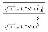
Fig. 1.16.1. Fractional meters

Mathcad gives the following result: square root from liter yields several meters in the first power, i.е. simple meters. This exercises thoughtful users, who understandably conclude that Mathcad does not work correctly with dimensions[71]. But the point here is that Mathcad rounds off units of measure to an integer power. If we put in the result another unit of measure (meter in power 3/2), then everything will be in order (see above).

But only Mathcad 2000[72] rounds off to integer number – earlier versions (Mathcad 8, for example) gave fractional powers of units of measure (m^1.5, for example, if we return to the example above). Mathcad’s developers considered that fractional power of unit of measure is «boots lightly». But it is not quite so. We can, for example, measure length in gallons (unit of volume), from which we have extracted the cube root. Why not! If there is a unit of volume cubic meter, then unit of length is possible – cubic root from gallon (liter, stere[73] and other units of volume – see fig. 1.16.2).

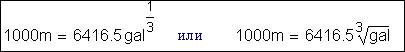
Fig. 1.16.2. Fractional gallons

Once there was a person who measured a room in bottles (0.25 litre bottles of vodka), but then tried to calculate the area in «square litres»[74]. He was not far from truth (see fig. 1.16.3).

Fig. 1.16.3. We measure square with help of volumes

The liter or «bottle» will serve as a unit of square, if we apply to them the corresponding fractional power (two thirds). Strictly speaking, there is nothing special in fractional units of measure. If, for example, in the CGS system we decompose ampere in terms of the system’s units:

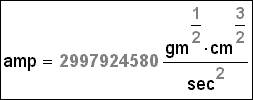
Fig. 1.16.4. Ampere in CGS

17. Units in user’s and special functions of Mathcad

Barometrical formula and graphs of change of pressure by altitude are shown in fig. 1.12.1. They also feature in one of the stories by Mark Twain[75]. It was in mountains and the talk was about how boiling water could tell altitude above sea level. The heroes of the story reminded for a long time that it is necessary to pull down in boiling water – thermometer or barometer. There was no thermometer to hand so they pulled down the barometer that broke at the same time. They pulled down another barometer – effect was the same. So our heroes could not define altitude above sea level but they learned to cook perfect «barometer soup».

Seriously to investigate the plots of Mark Twain – the work is senseless. But we take chances.

It was enough to carry testimonies of barometer to ordinate of the graph in (certainly, they did not have to pull down water) fig. 1.12.1, for heroes of Mark Twen, this way they could know the altitude above sea level. Certainly, to boil thermometer it was worth only in the case if they did not have the barometer.

Fig. 1.17.1. Determination of altitude by the temperature of boiling water

In the fig. 1.17.1 is shown how in Mathcad one can determine the altitude above sea level with help of temperature of boiling water (the problem from the story of Mark Twain). For it one barometrical formula is not enough. We also need the formula (function), connecting temperature of boiling water with atmospheric pressure. This function has the name wsp_pst and is included in the list of function of thermalphysic properties of water steam developed in Moscow Power Engineering Institutе [76]. In Mathcad-document in the fig. 1.17.1 by the first line the Reference is made to file with the name WaterSteamPro.mcd, where these functions are formed. After this reference in work it is necessary for work user’s function become available («visible»). These functions return the parameters of water and steam. For this comfort work with these functions it is made so that they were described in «Master Functions» of Mathcad. The file with the name Systems of units.mcd, reference is made too, keeps user’s units of measure.

Programs for calculation of properties of water and steam are developed a lot. The peculiarity of the WaterSteamPro is that that incoming in it functions have dimension arguments and return dimension values. It is very convenient for solving problems.

The files WaterSteamPro.mcd and Systems of units.mcd one can copy from Internet-to the address http://twt.mpei.ac.ru/orlov/watersteampro on the condition shareware[77].

But we repeat once more, the serious analysis of the problem about the altitude above sea level – it is «serious» enough work. Point is that that the barometrical formula is designed only for ideal gas. Apart pressure of air on the same altitude may vibrate much. And one more fact: temperature of air we decided 5 degrees Celsius, but it changes with the altitude.

But the main purpose of our calculation is not analysis of the story by Mark Twain but it is demonstration of possibilities of Mathcad for solving «dimension» problems.

We ought to note that not all built-in function of Mathcad work right with dimension arguments. Such mistake has been shown in the fig. 1.2.8. And here real mistakes during solving one of the most popular engineering problems are shown – conversion data from the table to some formula by different statical methods. In this case one usually use either interpolation, or smoothing by the method of least squares.

In the fig. 1.17.2 search of the coefficients a and b of the equation y(x) := a+b x (linear problem) is shown, smoothing the tabular data keeping in the vectors X and Y does it.

Fig. 1.17.2. Linear approximation

As we can see from fig. 1.17.2, the functions intercept and slope correctly work with dimensioned initial vectors – the functions intercept and slope have returned the coefficients а and b with correct dimension (m and m/kg). But despite correct values for the function line (input in Mathcad 2000), the coefficient a returns an incorrect dimension (m/kg instead of m). This mistake can be corrected by writing a := a × kg. into the Mathcad-document at fig. 1.17.2.

In fig. 1.17.3, a universal method is shown for smoothing tabular data with any dimensions by any formula with any number of coefficients[78]]. Initial data is kept in a matrix (table), but not in two vectors (see fig. 1.17.3). Part of this matrix is discrete values for the first argument (for example, length in metres ), but there is also a discrete value for the second argument (mass in kilograms). The third argument (density in grams by litre) depends on these two dimension arguments.

Fig. 1.17.3. Universal method of the regressive analysis of dimension data

Note that blanks in the table at fig. 1.17.3 are not empty data[79], but data where zero with invisible type is written (in white and white). These zeros[80] are ignored when we transfer data from the matrix M to three vectors X, Y and Z. (see the range with name From M to X, Y, Z in the fig. 1.17.3). Then the solution of the problem is reduced to minimization of the criterion function with name S(D^2), which address the heart of the problem: sum (S) of squares (^2) of deflections (D) of the sought line or surface from the data points.

The second method for forming a functional dependence by discrete points is based not in smoothing (approximation – see fig. 1.17.2 and fig. 1.17.3), but in interpolation. If we speak about spline interpolation then we have to establish that corresponding built-in functions of Mathcad cannot work with dimensioned arguments. The way out of this situation is shown in fig. 1.17.4.

Fig. 1.17.4. Spline interpolation of dimensioned tabular data

Spline interpolation, whose peculiarities of realization are shown in fig. 1.17.4, has one imperfection – the table must have no blanks. If there are some blanks then we can recommend smoothing (approximation) of tabular data by a given formula with the help of the least squares method (fig. 1.17.3), but not interpolation.

Very often we have to keep initial data for calculation in a table – in an Excel work sheet, for example[81][. Excel as a tabular processor gives user much more convenience than Mathcad, when working with matrices. But there is no technology of work with dimensioned values in Excel; neither can they be kept in Mathcad massifs. In fig. 1.17.5, fig. 1.17.6 and fig. 1.17.7 the solution of this problem is shown (units of measure disparity between Mathcad massif and Excel table).

Fig. 1.17.5. Work with dimension values kept in a Mathcad matrix

The following problem is solved in fig. 1.17.5: a user shows a type of some material (variable Type) and number of products (variable n), but Mathcad returns the price of the product (variable Price). The problem of «different dimension» of elements is solved in this way: dimension in the massif is present as commentary (left column of the matrix M), but out of matrix given matrix is added to elected elements.

Fig. 1.17.6. Work with values having different dimensions held in a Mathcad matrix

In fig. 1.17.6 two Excel tables handle data and output for a Mathcad-document, the result of calculation being introduced. In the fig. 1.17.7 these tables «are set off» by Excel tools.

Fig. 1.17.7. Excel’s tables in Mathcad

Built-in variables of Mathcad, that are «attached» to units of measure of physical values

Physical value	Unit of measure (proposed variable of Mathcad)
Activity	Bq
Time	day, hr (hour), min, s, sec and yr (year)
Dynamic viscosity	poise
Kinematic viscosity	stokes
Pressure	atm (standard atmosphere), in_Hg (inches of mercury), Pa, psi (pound force per square inch) adn torr (millimeters of mercury)
Length	cm, ft (foot), in (inch), km, m, mi (mile), mm and yd (yard)
Dose	Gy and Sv
Capacitance	F, farad, mF, nF, pF and statfarad
Charge	С, coul (coulomb) and statcoul
Inductance	H, henry, mH, mH and stathenry
Magnetic flux density	gauss, stattesla, T and tesla
Substance	mole
Magnetic flux	statweber, Wb and weber
Мass	gm, kg, lb (pound), mg, oz (ounce), slug (pood), ton (British ton) and tonne (metrical ton)
Power	hp (horse-power[82][82]), kW, W and watt
Magnetic field stress	Oe and oersted
Volume	fl_oz («liquid» ounce), gal (gallon), L, liter and mL
Illumination	lx (lux)
Area	acre and hectare
Potential	kV, KV, mV, statvolt, V and volt
Conductance	mho, S, siemens and statsiemens
Force	dyne, kgf, lbf, N and Newton
Luminosity	cd (candela)
Luminous flux	Im (lumen)
Velocity	kph (kilometre per hour) and mph (miles per hour)
Resistance	KW, MW, ohm, statohm and W
Temperature	K and R
Current	A, amp, KA, mA, mA and statamp
Angular	deg, rad and str (steradian)
Acceleration	g (free fall acceleration)
Frequency)	GHz, Hz, kHz, KHz and MHz
Energy	BTU (British caloricity unit[83][83]), cal, erg, J, joule and kcal

Some units of measure of physical values were taken from people’s names, in particular:

A.M. Ampere (1775-1836), French scientist, member of Parisian АN (1814), foreign member of Petersburg Academy of Sciences (1830), one of founder of electrodynamics. He was home educated. His main work is electrodynamics. He is author of the first theory of magnetics. He offered the rule for defining the direction of effect of magnetic field to magnetic arrow (Ampere’s rule). He carried out some experiments on investigation of interaction between electric current and a magnet. For these purposes he constructed many of devices. He discovered the effect of Earth’s magnetic field on a movable current conductor. He discovered (1820) mechanical interaction of currents and determined the law of this interaction (Ampere’s law). He reduced all magnetic interactions to interaction concealed in bodies circular molecular electric currents equivalent to flat magnets (Ampere’s theorem). He asserted that a big magnet consists of a huge number of flat magnets. Logically he developed the purely current character of magnetics. He discovered (1822) the effect of a coil with current (solenoid). He gave his view on equivalence of a solenoid with current and permanent magnet. He suggested a metal core of soft iron to increase magnetic field. He gave his view on use of electromagnetic effect for information transmission (1820). He invented commutator, electromagnetic telegraph (1829). He formulated the notion of “kinematics”. He also carried out investigations in philosophy and botany.

A.A. Becquerel (1852-1908), French physicist, discovered (1896) natural radioactivity of uranium salt. He received the Nobel Prize (1903, jointly with P. Curie and М. Складовской-Curie).

B.E.Weber (1804-1891) German physicist. He was foreign member of Petersburg Academy of Sciences (1853). Jointly with Gauss he worked out the absolute system of electric and magnetic units.

A. Volta (1745-1827) Italian physicist and physiologist, one of the founders of teaching on electricity. He created the first chemical source of current (1800). He discovered contact potential difference.

K.F Gauss (1777-1855) was a German mathematician, foreign Corresponding Member (1802) and honorary foreign member (1824) of the St. Petersburg Academy of Sciences. Characteristic feature of the scientific work of Gauss is limited connection between theoretical and applied mathematics and breadth of problems. The Gauss work had a great influence on the development of algebra (proof of the main theorem of algebra), theory of number (square-law residue), differential geometry (inner geometry of surfaces), mathematical physics (the Gauss principle), the theory of electricity and magnetism, geodesy (working out the method of least squares) and many parts of astronomy.

J. Henry (1797-1878), American physicist. He created powerful electromagnets and the electric motor, discovered (1832, independently of M. Faraday) self-induction, and determined (1842) the intermittent character of condenser discharge. He was the first manager (1846) of the Smithsonian institute.

G.R.Hertz (1857-1894), German physicist, one of the founders of electrodynamics. He experimentally proved (1886-89) the existence of electromagnetic waves (using the Hertz chopper) and identified the main properties of electromagnetic and light waves. He made the Maxwell equation symmetric. He discovered the outer photoemissive effect (1887). He formulated mechanics free of the notion of a force.

S. Gray (1666-1736), English physicist. He discovered in 1729 the phenomenon of electroconductivity. He determined that electricity may be transmitted from one body to another one by metallic wire or spinning thread, but it can not be transmitted by silk thread. He was the first who divided all substances into conductors and nonconductors of electricity.

J.P.Joule (1818-1889), English physicist. He experimentally proved the law of conservation of energy and determined the mechanical equivalent of heat. He determined the law that was called the Joule and Lents law. He discovered (jointly with U. Tomsone) effect that was called the Joule and Tomsone effect.

G.R. Sievert, Swedish scientist.

U. Kelvin - Tomsone (for his scientific services in 1892 he got the title of Baron Kelvin) (1824-1907), English physicist, member (1851) and president (1890-95) of the Royal Society (London), foreign Corresponding Member (1877) and honorary foreign member (1896) of the St. Petersburg Academy of Sciences. He did work on many parts of physics (thermodynamics, theory of electric and magnetic phenomena, etc.). He gave one of definition of the second law of thermodynamics and offered the absolute scale of temperature (Kelvin scale). He experimentally discovered some effects that named after him (the Joule and Tomsone effect). He was an active contributor to realization of telegraphy by transatlantic cable and determined the dependence between oscillation period of a circuit, its capacity and its inductance. He invented many electro-measuring instruments and perfected some sea-going instruments.

C-A de Coulomb (1736-1806), French engineer and physicist, one of the founders of electrostatics. He investigated the deformation of a lisle thread and discovered its laws. He invented (1784) the torsion balance and discovered (1785) the law named after him. He determined the laws of dry friction.

I. Newton (1643-1727), English mathematician, mechanical engineer, astronomer and physicist. He is the creator of classical mechanics. He was member (1672) and president (since 1703) of the Royal Society (London). His basic works are «Mathematical Principles of Natural Philosophy» (1687) and «Optics» (1704). He worked out (independently of G. Leibniz) differential and integral calculus. He discovered dispersion of light, chromatic aberration, and investigated interference and diffraction. He developed a corpuscular theory of light and advanced a hypothesis about corpuscular and wave properties of light. He built a reflecting telescope. He formulated the main laws of classical mechanics. He discovered the law of universal gravitation, developed the theory of motion in heavenly bodis and created the basis of celestial mechanics. He considered space and time as absolute. Newton’s works were greatly ahead of the common scientific level at that time and were obscure to contemporaries. He was the manager of the Royal Mint and arranged monetary business in England. He was a well known alchemist. Newton was engaged in ancient kingdoms chronology. He devoted theological works to interpretation of biblical prophecy (many of these works have not been published).

G.S.Ohm (1787-1854), German physicist. He determined the main law of electric circuits (the Ohm law). Also worked on acoustics and crystal optics.

B. Pascal (1623-62), French mathematician, physicist, religious philosopher and writer. He formulated one of the main theorems of projection geometry. He also did work on arithmetic, theory of number, algebra and probability theory. He constructed (1641, or according to some sources 1642) a digital arithmetic machine. One of the founders of hydrostatics, he determined its main law. He also worked on the theory of air pressure. From 1655 he lived an almost monastic life. Polemics with Jesuits were reflected in «Provincial Letters» (1656-57), a masterpiece of French satirical prose. In «Thoughts» (published in 1669) Pascal developed notions of the tragedy and fragility of man, situated between the abyss of infinity and nonentity (man is a «thinking reed»). He saw the mastering of the mysteries, and escape of man, in Christianity. He played a vital part in the formation of French classical prose.

G. L. M. Poiseuille (1799-1869), French doctor and physicist. Works on the physiology of breathing and the dynamics of blood circulation. He was the first (1828) to apply a mercury manometer to measurement of blood pressure in animals. He experimentally determined the law of outflow of liquid.

U. J. M. Rankine (1820-1872), Scottish engineer and physicist, one of the creators of technical thermodynamics. He offered the theoretical cycle of steam engine (the Rankine cycle), temperature scale (the Rankine scale) – with a zero point coinciding with zero of thermodynamic temperature but with a Rankine degree (°R) that equals ⁵/₉ К.

E. V. Siemens (1816-1892), German electrical engineer and industrialist, foreign Corresponding Member of St. Petersburg Academy of Sciences (1882). The founder and main holder of electrotechnical concerns. He created an electro-machine generator with self-excitation (1867) etc.

J. G. Stokes (1819-1903), English physicist and mathematician, member (1851) and president (1885-90) of the Royal Society (London). He had basic investigations on hydrodynamics (the Naviye-Stokes equation, the Stokes law). He also had works on optics, spectrography and luminescence (the Stokes rule), gravimetry, vector analysis (the Stokes formula).

N. Tesla (1856-1943), inventor in the field of electro- and radio engineering. Serbian by birth, he lived in the USA from 1884. In 1888 he described (independently of Italian physicist G. Ferrarissa) the rotary magnetic field phenomenon. He worked out multiphase electric machines and schemes of distribution for multiphase currents. He was a pioneer of high-frequency technical equipment (generators, transformer etc, 1889-1891). He investigated the possibility of transmitting signals and power without wires.

E.Torricelli (1608-1647), Italian physicist and mathematician, a pupil of G. Galilei. He invented the mercury barometer, discovered the existence of atmospheric pressure, and vacuum. He derived a formula that bears his name.

J.Watt (1736-1819), English inventor, creator of the universal heat-engine. He invented (1774-84) the steam engine with the double-acting cylinder where he applied a centrifugal governor, transmission from the cylinder’s rod to a parallelogram balancer, etc. (patent 1784). The Watt engine played a vital role in the development of engine production.

M. Faraday (1791-1867), English physicist, founder of teaching about electromagnetic field, foreign honorary member of Petersburg Academy of Sciences (1830). He discovered the chemical effect of electric current and the relation between electricity and magnetism, magnetism and light. He discovered (1831) electromagnetic induction – the phenomenon that formed the basis of electrical engineering. He determined (1833-34) the laws of electrolysis that were named after him. He also discovered paraparamagnetism, diamagnetism and rotation of a plane of polarization of light in a magnetic field (the Faraday effect). He proved the identity of different types of electricity. He introduced the notions of electric and magnetic field and suggested the existence of electromagnetic waves.

H.K.Orsted (1777-1851), Danish physicist. Foreign honorary member of Petersburg Academy of Sciences (1830). Works on electricity, acoustics and molecular physics. He discovered (1820) the magnetic effect of electric current.

Historical and political commentaries to this table

1. One speaks: «Great man», picking him up from croud. But if one looks at the table, he can say that the highest appraisal of a scientist if his name people are written with small letter: newton, volt, ohm, joule, kelvin and so on – if unit of measure of physical values were named of his name[84]. (Other people have possibility to become famous for units of measure but these units are not physical one – to decorate coin or bank not of their portraits.)

2. The science connecting with units of measure of physical values is named metrology. Metrology – it is only one part of physics which name has three adjectives[85] but not two ones: except theoretical and practical metrology there is legislative metrology[86]. All historical cataclysms, as rule, were accompanied by radical changes in the system weights and measures. Great French Revolution gave us near calendar, metrological system (gram, litre, stere) and many other things. Certainly many things sank into oblivion but many things kept. Civil war in Switzerland in 1847 flamed up owing to religious and metrical. Seven edgings struggled for their own system weights and measures. If Swiss struggled for it then one can understand all importance of weights and measures in life of single man and all society[87]. But last century in Russia old and new units of measure of length and mass (weight) lived more or less in harmony. But we needed «fundamental» October Revolution for vershoks, arshines, sazhens, versts and a lot of other things «sank into oblivion». Now British system measure lives its last days (years). Anglo-Saxon (including Americans) willy-nilly are forced to use SI. First of all it connects with universal economic integration. For example, the fact, that there is no «American» in SI, very confuses of Americans – pascal, farad, coulomb, gauss, tesla, henry, hertz, kelvin, celsius, joule, watt, ampere, volt and etc. – these are all «Europeans»[88]. «Metrical» resistance the Old and the New World and told on that that Americans, for example, hardly acknowledged German Ohm (ohm – units of electric resistance), but bluntly refuse to acknowledge another German Siemens (siemens – unit of electric conductivity). But why businessman and inventor Siemens is better than their American colleagues Bel and other[89], for example. Americans measure conductivity in «mho»: mho – it is palindrome from «ohm»[90] but not in siemens. When SI was discussed Soviet delegation insisted on that that there were Russian in list of units but not only English, French, Italian and German – it is suggested to measure gas constant (see fig. 1.12.1) in mendelevium. But this suggestion was not accepted[91].

3. History of units of measure is history of pressing from everyday life «non-decimal» values. We compare: 1 verst= 500 sazhens=1500 arshines=24000 vershoks[92] and 1 km=10³ m=10⁴ dm=10⁵ cm=10⁶ mm. The same story happened with money[93] – we remember how English «bewailed» their «old, kind» crowns (5 shillings), quineas (21 shillings), shillings (12 pences or 1/20 of pound) and so on. But only time and angles do not give in to these changes: (there are 24 hours in day and night, there are 60 minutes in an hour, there are 60 seconds in a minute. There are 360 degrees[94] in a circle, there are 60 angular minutes or 3600 angular seconds in a degree).

[1] Account of a dimension often allows deriving formula. For example, vibration frequency of a pendulum depends on only the length of the pendulum (certainly we speak about simple pendulum) and free fall acceleration. From these conditions it is easy to derive the formula.

[2] Character of the flow of water in a duct (turbulence, laminarity) can be estimated by three different parameters: speed, diameter, and ductility. But we can do it also by one non-dimensionals parameter – by number Re.

[3] Good rule. If you solve «non-dimensionals» problem then it is better to turn off the mechanism of the work with dimensions. – see «radio-point» None in fig. 1.2.

[4] In the black-and-white pictures of the book these objects differ by print: formulas are straight print (Arial), commentaries are chopped one (Times).

[5] Here we work with scalar variable. In Mathcad it is possible to work with vectors and matrixes (massif). Massifs can keep dimension values too, but this value must be the same dimension.

[6] In Mathcad it is better to use operator of output numerical value «=», but not that operator. The main thing is that that if some variable F or any other one has already kept something, then thisто это «something» will be displayed. If this variable is «empty», then the operator «=» (output) will automatically turn into the operator «:=» (input – technology of SmartOperator). This way we insure against some mistakes that connected with overdetermination already definite variable.

[7] Good rule. First time one even the simplest one (m, for example) is worth to input with help of «Master dimensions», and then this one we should copy.

[8] Here s, but not sec is picked out as since Mathcad direct by default toward SI. If we change the system of units (see part 2), then instead of s, sec will appear. The second way of writing is better. First of all we can use it both for SI and for other three systems built-in in Mathcad. In the second place, we can mix up s capital with S title. S title in our calculation is a square in fig. 1.1.1 (Square and electrical conduction – siemen, frankly speaking).

[9] lb – libra (old French coin) pound. The word livra comes from Latin. In Latin it means rind of fixed tree where one wrote text. Another French word livre – book comes from this.

[10] In the fig. 1.1.1 we change both units and format of the number (1.307553 × 10⁵= 130755.3) – see label Number Format in the fig. 1.1.1. Here for better reminder numerator and denominator are worth to divide by unit of length lbft/ (ft²sec²).

[11] From fig. 1.1.2 we can see that the resulting force equals 0 kgf. Here, any units of force cannot be added – zero is zero in any units of any system. Students are criticized, when they add to zero some unit. But this rule does not apply when we work with the relative scale (see part 14). Also, we have to remember that in computing mathematics zero is not, as a rule, really zero but something close to zero: «almost zero in dynes», is not the same «almost zero in kilogram-force». So Mathcad adds right the unit of force to the result in the fig. 1.1.2.

[12] For instance, a user may forget that pascal is written with a capital letter (Pa), but torr with lower case (torr), even though both units of pressure are named after scientists who made great contributions to natural science – B.Pascal (1623-62) and Torricelli who invented mercury barometer (1608-1647).

[13] Or we can do it with the help of special user’s functions, if we are referring to relative measure scales and not absolute ones (see part 14).

[14] In Mathcad the variable g keeps the value of free fall acceleration. It is impossible to understand why, of all the physical constants, the program builders have only this one in Mathcad – especially as it is not constant: on the equator it has one value but on the poles another (see also part 5 «Unit with suffix»). If the program builders of Mathcad did it for some metrology laboratory, they did not accept this program, since g – is the legalized unit of mass.

[15] The operator м := m has a practical sense. The variable m is quite «popular» in calculations. We can write m := 20 kg (mass of some thing equals twenty kilograms) and… disrupt the value of the built-in variable m (unit meter). We have, incidentally, already disrupted the values of the built-in variables S (siemen) and F (farad) in the first example of this book (see fig. 1.1.1).

[16] It is usually off-system units which are nevertheless widely used in calculation. In calculation we can introduce dated units – see the second, «informal» part of the book.

[17] Certainly we can introduce this unit as atm := 98066.5 Ра, but our note is more obvious – we can see physical sense of technical atmospheres: kilogram force effected on square centimeters.

Good rule. Don’t change complex units to «short» ones without good reason, as you will hide the «physics» of the problem.

[18] Coming back to point 1, we can note that there are several ways to write some units built into Mathcad: L – liter, W – watt, J – joule, N – Newton and so on.

[19] We repeat (see preface), that it is difficult to thnk of a scientific and technical region where we use pascal without any factors. In the region of low pressures everybody does without the pascal altogether - they change them by millimeters of mercury or millimeters of water.

[20] Keeping files off-system and dated units (see the tables 3.16-3.17 in the third part of the book), can be «skimmed» from ftp-server using the address: ftp://twt.mpei.ac.ru/ochkov/units. There you can find the files with problems from this book and some others.

[21] Good rule. Some units are worth duplicating: квт·час:= kW·hr kW·hr:= kW·hr and so on – we allow user to choose which is the more convenient. It is better if we write unite in different languages: bbl := 42 gal баррель := bbl and so on.

[22] One such «factor» in Mathcad is built in: % = 0.01, but we discuss this below – in part 6 «Non-dimensionals units».

[23] Such defects, or rather ambiguities, are inherent in SI. One more example: J is the designation of dimension of force of light and unit of energy (labor) joule.

[24] There is a well-known equivalent philological paradox: a comma in the order sharply changes the sense. It depends on where we put this comma. And here is the similar metrological paradox: a unit of mass mkg changes its «weight» (or rather mass), depending on where we put invisible sign of multiplication – mk?g: microgram, 10^-9 of kilogram or m?kg:мmilli-kilogram, i.е. it is gram. The first interpretation (or rather «in general») is more widespread. But if we take into account that the main unit of mass is kilogram (kg) but not gram (g) and m is the generally accepted factor (milli, 10^-3), then duality of the interpretation mkg becomes possible. This given example shows that kilogram is not good as the main unit of SI – from the beginning it was complex one (kilo and gram). In our example it is better to write μg (μ was not written earlier, since there was no such Greek letter on printing machines), but not mkg.

[25] When the author went to school the International system (SI) was hard taken root in subject «Physics». In this connexion it was considered (as joke or seriously) that in a shop you had to ask a vendor to weigh not 200 grams of sausages but two Newtons - as since weight is mass but not force!

[26] Actually, when we print such a Mathcad-document, the blank between suffix (or prefix – see the part 4 «Factors before units») will appear once more: kgf ? kg f. The multiplication sign will appear on the display between factors (see fig. 1.5.1), if we lead the cursor to a complex variable.

[27] About «sly» unit of mass mkg you can see above in the part 4 «Factors before units».

[28] Unit is unit, but unity is a number.

[29] As the reader will understand, the mole is a measure of something that has a number of base units that equal Avogadro number (6.022 10²³). Starting from this we can determine a unit that we call thing: thing := mole/6.022 10²³. But in this case the «physics» of the problem (integer) will clash with its «mathematics» (real variable thing).

[30] For example, it is impossible to sum percents and degrees of arc. But Mathcad allows to us to do it since percent and degree are both simple numerical constants:
% + deg = 0.027 % + deg = 2.745 % % + deg = 1.153 deg.

[31] Gram-mole (g-mole) is a dated designation of mole. But milligram-mole (mg-mole) is one-thousandth of mole. Here it is better (more correct) to write mmole, but chemists cannot be «made over». We have «the same story» with gram-equivalent that is mole too.

[32] The given «non-dimension» unit is named in honor of J.Napier (Napier – 1550-1617). He was Scots mathematician and the inventor of logarithms.

[33] This base is chosen to show once again the convenience of calculation in Mathcad with user units: a human heart pumps on average 70 milliliters per second in the time of normal мл крови в секунду при нормальном (middle) pressure 120 on 80 millimeters of mercury.

[34] The operator, determinative of this function, «lies» on the colored background for we can see the name of the function. When we call this function as a prefix operator there is no colored background. That’s why user sees not dB p = 5 dB, but p = 5 dB (dB after a numerical answer the user prints in addition himself: the constant dB equals one and he does not change anything in the answer, simulating only unit).

[35] Here one should remember that Mathcad may display not an absolute value of zero, but an approximate one. In this case zero kilogram and zero microgram are not the same thing.

[36] We can connect rubles with seconds if we give material form to that famous principle: «Time is money». But we already have time in our calculation when we look through the payment for electric power in the fig. 1.7.1. Besides, almost all derivative units use time (see the tables 3.6-3.9 and 3.11-3.14 in the third part of the book). But luminous intensity is a solitary value that we can see only in the table 3.10. Author has not yet seen a Mathcad-document yet where candela is used. We can say that SI has three values of different kind: the first kind is mass, time and distance, the second kind is current and temperature, and finally the third kind is amount of agent and luminous intensity.

[37] Candela (in Latin it is candle) is the unit of luminous intensity (SI). In our «electrotechnical» calculation we can use it as since power of lamps was measured in candles but not in watt.

[38] For example, if in the point 1 in the fig. 1.7.1 is to write $US = 28 roubles, then we can get the payment for electric power $ US. The number 28 we can change to some constant. The value of this constant is compared with data from Central bank. This way our calculation will be more efficient and accurate.

[39] Author could not at all understand one technicoeconomic calculations, where there was a mistake. It was localized only after the operator rouble := 1 was changed to the operator rouble := cd. It turned out that in one formula roubles was summed with non-dimension value. After interchanging rouble := 1 to rouble := cd realization of the operator with the faulty formula was interrupted by diagnostic message for error «Variance in physical values».

[40] Economists object reasonably enough that price and cost are different notions that many of us mix up. But it looks like the radius and diameter of circle – the units used will be for distance. The author does not know the name of a new dimension value that relates to price and cost, but the reader will understand what we are talking about.

[41] We’ll interpret «the same format» variables as the variables of which names have the same color, type, dimension and other attributes of type.

[42] Attributes of the type of the styles of Mathcad-document Russian user has to change at once as the built-in styles do not support Cyrillic alphabet. You can make this change with the help of the Equation command… in the menu Format. After this turning on the work with Cyrillic alphabet, it will be rational to save the given Mathcad-document as template (form) either with name Normal (then, on starting up Mathcad we’ll be accompanied by appearance of russified form) or with some user’s name («My document», for example). Such form (and others built-in in Mathcad: Blank Worksheet, bookone, calcform, contents, report and specform) are called with help of the command New… from the menu File. This technology with templates lies at the heart of many Windows applications – for example, in Word.

By the way we speak about Word or rather about the text editor that is built in Mathcad. We should note those text commentaries in Mathcad-document can be picked out by styles: general text, titles of different level and so on.

[43] Units that are output on the Mathcad system display itself, have style Constants, but not Variable, а: 100 cm = 1 m – here cm (the style Variable) user has introduced into, but m (the style Constants) has been output automatically.

[44] «Why not!» – «Почему бы и нет!»: в выборе переменных пользователь «хозяин-барин». Но переменным (величинам), конечно, лучше давать те имена, которые рекомендованы SI (see таблицы 3.4, 3.6-3.9 в третьей части книги) или которые закрепились за ними в процессе развития той или иной научной дисциплины.

[45] У пользовательского стиля можно менять название, а у встроенного – нет. Разным стилям можно дать одинаковые названия. Эту особенность Mathcad можно считать и ошибкой, и средством создания разного рода «программистских трюков».

[46] In the report in the fig. 1.9.1 the variable blue has blue color, but the variable black has black one. It is possible to be more original: to introduce into calculation two variables of the same name cloth with different color – one blue, one black.

[47] Or rather it is not Mathcad, but Maple – in Mathcad kernel of symbolic mathematics from Maple is built in. Is that so it is possible to read giving the command «О Mathcad» in the menu «Help»: ©1986-1999 MathSoft, Inc. All rights reserved. Mathcad and Axum are registered trademarks and MathConnex, QuickPlot, Live Symbolics and IntelliMath are trademarks of MathSoft Inc. U.S. Pat. Nos. 5,469,538 and 5,526,475. SmartSketch LE ©1997-1999 Intergraph Corporation. Volo View Express ©1999 Autodesk, Inc. International CorrectSpell software ©1993 Lernout & Hauspie Speech Products N. V. MKM (MathSoft Kernel Maple) ©1994 Waterloo Maple Software. Microsoft Internet Explorer ©1995-1999. Copyrights on symbolic mathematics are underlined by thick type.

[48] «If you do not know Ohm’s law – you must stay at home!»

[49] There were and are versions of Mathcad for Unix, Mac and other operation systems. In our book, however, we speak about versions of Mathcad for Windows.

[50] T, by the way, is a factor for forming decimal divisible units of measure (Т – tera, 10¹²).

[51] With help of the Mathcad function time one can fix the fulfilment speed of some operators and operators blocks. For example:

[52] Here the control of dimension without using programming means is shown. In Mathcad-programs it is possible to simplify such control (see fig. 1.27).

[53] In this sense such an operator d := d may be strange. However in Mathcad this operator is regular enough – it deprives the variable d of its numerical value for the next symbol conversion (see part 9 «Symbolic mathematics and units of measure»).

[54] It is illuminated in the fig. 1.12.1: in a Mathcad-document, by changing the background color of some operators one can direct attention to them. The calculation is simplified more than is realistic – we use the formula for ideal gas. Apart from this, we do not take into account the behaviour of air temperature by height. The value of the gas constant is transferred from the Mathcad reference book (not only physical constants but dimension ones are kept there) to the variable R. There are three «metrological» remarks about the variable R. First of all, as we assumed the variable to be the value of the gas constant so we … spoiled degrees Renkin (see the part 14 «Relative scales of measure»). The solution of this problem – see the part 8 «Styles of variables and units of measure». In the second place (experts suggested it but the developers of SI did not accept) this constant must be equated to one and the value of joule and other units of energy must be adjusted accordingly. And in the third place, during the conference where SI was asseverated, the Soviet delegation suggested to give to the complex unit by which we measure the gas constant the name - mendelevium.

[55] During critical analysis of units of measure of physical values, a feeling grows that somebody has deliberately mixed everything up: mm of mercury is the unit of pressure but not length. The list of such nonsense we can continue: light year is not time but distance (towards stars as rule), horse-power is not force but power, pound sterling is not mass but cost, and so on.

[56] In such tank the volume of the liquid residue is measured by old «grandfather’s» way: from the upper hatchway one toughs by the stick the bottom and then he measures the length of the wet end of the stick.

[57] Here it is possible to use the built-in function UnitsOf, returning unit of measure of its argument. But the dimension control mechanism realized in the program in fig. 1.1.13 is easier and more obvious. Also we should not forget that the function UnitsOf is introduced only in Mathcad 2000. The dimension control method for values input into the calculation used in fig. 1.13.1 we have already described in the part 11 «Control of dimension».

[58] Short advice that appeared when we started up Mathcad for the first time: «Did you know…». As rule users remove the tick near the note Show tips on startup. One knows English badly, another considers that «To teach the erudite is only to spoil him». But most people want to start the solution of their problem as soon as possible. They are afraid «to frighten off» their incipient ideas. Abstract advices stand in the way between the idea in the user’s head and its display...

[59] The Add Line operator method for the matrix is not a commodity. But we repeat once more that it is not considered a commodity method to use units of measure in programs too.

[60] The word «Pro» in the title means «Professional». Such version Mathcad is managed of programming tools.

[61] The «American» analogue of Kelvin is: K = 1.8 R.

[62] the author once saw a telecast of the Discovery channel. This channel excels in interesting plots but very bad translation of the text into Russian. On day an announcer said «that fuel must be cooled to minus 400 degrees». This phrase immediately generated perplexity, and only later did I understand that the announcer referred to degrees Fahrenheit.

[63] Scale may be both for temperature and for pressure: there is absolute pressure, but there is excess pressure about atmospheric, for example. As a rule all manometers are graduated for excess pressure. One more example of excess value – the growth of a man, measured in vershoks (see the example 3 in the second part of the book).

[64] This phrase we can repeat with respect to Fahrenheit degrees: the Fahrenheit degree equals the Rankin degree, but the Fahrenheit scale is moved relative to Rankin by 459.67 degrees (Fahrenheit or Rankine).

[65] There is no «degree» symbol on a keyboard. This symbol is either input using the Alt+0176 chord or copied from Mathcad’s set of mathematical symbols.

[66] For we can see on the display that it is possible to change the background color from white to blue, for example. For solving the metrological problem we have already used the invisible operator (see fig. 1.6.3). Here is one more example of using invisible symbols during work with dimension values. A zero dimension value is output by the Mathcad operator then corresponding units of measure hidden, writing it in white-on-white (compare: 1 m - 100 cm = 0 m and 1 m - 100 cm = 0).

[67] It is the third «stumbling-block» when we work with dimension values in Mathcad. The first two «stumbling-blocks» are Fahrenheit degrees and degrees Celsius (see the part 13 «Dimension in programs») and programming (see the part 14 «Relative scales»). As these «blocks» users often refuse from the work with dimension values in Mathcad one of the purposes of this book – to teach reader avoids these «reef stumbling-blocks».

[68] Reader can not penetrate into main point of the problem (it is calculated the heat transfer coefficient during boiling water α depending on pressure p and heat demand q) – it is enough to understand the mechanism of using dimensions in it.

[69] As rule all coefficients must be non-dimensional. But in single scientific discipline one refuse sometimes from this rule.

[70] Author could show concrete example from «his » formulas, but he is afraid that they are not clear enough for reader.

[71] We can see such a peculiarity in fig. 1.15.2, where powers of meters and kilograms were zero: kg⁰ m⁰ s^-2. As a matter of fact fractional powers must be there.

[72] It actually the first «patch» PROmc2k1.exe (3.5 MB). Updated version of Mathcad 2000, denoted by the letter A, will work correctly with powers of units – it stops to round them off to integer number. The question of dimension with additional power remains open.

[73] Volume of a cube with edge of 1 m.

[74] With this example we look ahead by a few steps – its place is in the second part of the book.

[75] Author can not remember what the story was where that episode was described. And it may be this was not written by Mark Twain at all!?

[76] The base of universal power engineering is heat-and-power engineering. Working substance of the cycles in thermoelectric power station and atomic power station, as rule, is water or water steam.

[77] User gets only share of the program (ware). User gets full programs after fulfilment some conditions.

[78] The word «any» is used three times in the sentence. Certainly some limitations that connect with limitations of the built-in function Minimize can take place in the given problem.

[79] Mathcad, unfortunately, can not work with sparse matrices.

[80] It is considered that there are no zero values among initial data. If this is not so, then we can change zeros to infinity or some other value that does not occur in the table.

[81][81] Developer of Mathcad underline that this program leads own family tree from tabular processor. The main difference of the technology of calculations between Mathcad and Excel is that in Mathcad the symbol «=» is put after mathematical expression, but in Excel – before.

[82][82] Besides standard horse-power (hp) in Mathcad, there are other «horse» units of power, that are used in Great Britain and North America – bhp («boiler kettle» horse-power), ehp («electric» horse-power), mph («metrical» horse-power), hpUK (British horse-power), whp («water» horse-power) and etc.

[83][83] Apart from BTU in Mathcad, there are other caloricity units used in Great Britain and North America – BTU15 (unit attached to water when temperature is 15 degrees Celsius), CBTU (Canadian caloricity unit), IBTU (caloricity unit of the international agency of standards agency, ISO), mBTU (the «main» caloricity unit) and tBTU («thermodynamic» caloricity unit). In addition to Mathcad’s standard calorie cal, other caloricity units are built in – cal15 (unit attached to water when temperature is 15 degrees Celsius), cal20 (unit attached to water when temperature is 20 degrees Celsius), dcal («dietetic» calorie), mcal (the «main» calorie) and tcal («thermodynamic» calorie). People have become confused by all these calories and have decided to begin from a blank sheet – from joules.

[84] About such people everybody say «he were the smartest man in the world!» – we’ll be back to span in the second (informal) part of the book.

[85] The adjectives of scientific disciplines are harmed a little. We try to illustrate it by next dialogue: «Who built this tower?» – «Engineer Shukhov did». – «Is he like our mother engineer?» – «No, my son, our mother is chief engineer». On the other hand «present» scientific disciplines are not afraid the adjective «amusing»: amusing mathematics, amusing physics and so on. The adjective «amusing» we can regard as test stone. If we joined it (the adjective) to the name of discipline and you understood that where there is no amusing (humor), there is no real science. But it is very difficult to draw an accurate distinction between science and pseudo-science: mathematics, physical mathematics (in the sense «physical and mathematical sciences»), physical chemistry, chemical chemistry, theoretical chemistry, applied chemistry and, finally, alchemy (metaphysics). So we fluently pass from science to pseudo-science.

[86] If we remember about disputes that took and take place round nominal names of units of measure then we can speak about «political» (diplomatic) metrology.

[87] For example, in England holders of many pubs oppose… against input metrical system. Point is that the metrical system must change a pint (pt) to a half litre. Hence visitors will drink less:

[88] Exclusion that verifies the rule – henry is unit of magnetic induction that was called of name of «pure-blooded» American.

[89] There are units of measure of sound force decibel (one-ten of Bel), but it did not come in SI and does not consider unit of measure. It is some logarithmic factor.

[90] By the way the functions siemens and mho are built-in in Mathcad.

[91] Certainly Mendeleev is great scientific but what for we’ll be use so difficult word («mendelevium»).

[92] There is such line for memory dated units of measure of length: rifle three-line has caliber 7.62 mm; there are ten lines in an inch, there 7 inches or 4 versoks in a span, there are 16 vershoks in an arshine, but there are 3 arshines in a sazhen. One said that to remember the telephone number is very simple – 32-08: thirty-two teeth 8 fingers… Author hopes that reader has felt all delights (without inverted commas) of the metrical system.

[93] We can see the same situation in bank notes and coins: 1 kopeck, 2 kopecks, 5 kopecks, 10 kopecks, 50 kopecks, 1 rouble, 2 roubles, 5 roubles, 10 roubles, 50 roubles, 100 roubles, 500 roubles and 1000 roubles, if we speak about Russian system of measure of money, but not 1 kopeck, 10 kopecks, 1 rouble, 10 roubles and 100 roubles, as metrical money system requires. Here we can see the sign of magic numbers – almost all money systems all over the world (USA, Germany, Europe) are based on 7 bank notes.

[94] The famous computer «Spark-226» could work with radians, degrees and grads (there are 90 degrees and 100 grads in a right angle – one of the attempts of partial «decarisation» of angular measure). Built-in language of this computer by default calculated in radians, but this default could be broken by the command SELECT D (work with degrees) and SELECT G (work with grads). There was such joke: if a worker was away a few minutes then his colleague carried out the operator SELECT G. The program gave wrong results and the worker could not understand why.