A.P.Solodov.
Computer Model of Nucleate Boiling
In: Convective Flow and Pool Boiling :
Proceedings of the International Engineering Foundation 3rd Conference held at
DENSITY OF ACTIVE NUCLEATION CENTRES
AND FRACTAL NATURE OF THE SURFACE
COMPUTER MODEL OF NUCLEATE BOILING
Alexander
P. Solodov
Moscow
Power Engineering Institute (TU)
ABSTRACT
A computer model has been established for
nucleate boiling heat transfer in a wide range of pressure. The information on
nucleation centres density required in the model was
obtained using fractal representation of the rough heating surface.
INTRODUCTION
About nucleate boiling it seems that at least
the complete list of particular mechanisms is known; these are e.g.:
- the
bubble growth in superheated liquid,
- evaporation
of a thin liquid film under the bubble, and so on.
On this basis we attempted to construct a
computer model for the calculation, with the purpose to reproduce experimental
results in a wide range of parameters, particularly of pressure.
This model requires information on nucleation centres density.
We can get this information using
fractal representation of the rough heating surface (with fractal dimension up
to 3).
This technique is already used in
different areas - from drawing of realistic landscapes with computers, up to
investigation of polymers adsorption or electrochemical phenomena on rough
surfaces.
PHYSICAL
MODEL
Three characteristic scales exist at nucleate
boiling:
- critical bubble
radius , ![]()
- distance between the
active nucleation sites ![]() ,
,
- bubble departure
radius ![]() .
.
At intensive boiling the following relation
holds: ![]() . Bubbles by
the size
. Bubbles by
the size ![]() grow continuously because of evaporation.
After achievement of size L
, fusions occur with sharp changes of size.
grow continuously because of evaporation.
After achievement of size L
, fusions occur with sharp changes of size.
Earlier we considered statistics for the
similar process of growth and fusion at dropwise
condensation (Solodov and Isatchenko
(1967), Isatchenko, Solodov,
Maltsev, Jakusheva (1983)).
The main result is also used here, according to which the bubble population
with the sizes of order of distance L
between the centres is the most representative,
because at ![]() a maximum exists within the distribution
function for bubbles. Therefore, we can limit our analysis of growth to such
bubbles.
a maximum exists within the distribution
function for bubbles. Therefore, we can limit our analysis of growth to such
bubbles.
The heat flux q on a wall is set constant corresponding to
boiling with electrical heating.
In this case, temperature pulsations on the
wall take place. During a waiting time, the superheating increases up to a
level, when centres are activated. Further,
temperature of the wall is determined by evaporation of a film under the
bubble, by a possible movement of liquid in the external area of the bubbles,
and by exchange of liquid on the wall after fusions of bubbles.
The heat transfer model is designed from the
following elementary mechanisms:
¨Unsteady
heating of liquid during the waiting time in the domain ![]() , where x is
the distance from the nucleation centre. As the quantitative characteristics of
this process were used: superheat
, where x is
the distance from the nucleation centre. As the quantitative characteristics of
this process were used: superheat ![]() and enthalpy boundary-layer thickness on the wall
and enthalpy boundary-layer thickness on the wall ![]() .
.
¨Unsteady
heating or convective heat transfer outside the bubble, ![]() . The
movement of liquid is compelled by the growing bubble.
. The
movement of liquid is compelled by the growing bubble.
¨Formation
and evaporation of a thin liquid film under the bubble in the domain ![]() . Formation
and growth of a dry spot owing to evaporation of the liquid film under the
bubble near
. Formation
and growth of a dry spot owing to evaporation of the liquid film under the
bubble near ![]() .
.
¨Growth of
a half-spherical bubble in the layer of superheated liquid (![]() ). The heat
is brought to the bubble
). The heat
is brought to the bubble
- through the bubble
foot from the wall (q), and
- through the
spherical surface of the bubble (![]() ) from the
superheated liquid.
) from the
superheated liquid.
For
large bubbles, ![]() , the heat
flow from the superheated liquid occurs only near the bubble foot.
, the heat
flow from the superheated liquid occurs only near the bubble foot.
The application of this model permits to
calculate the space-temporary distribution of the wall superheat
![]() . The global
averaging further gives the average value of the wall superheat
. The global
averaging further gives the average value of the wall superheat ![]() and the average value of heat transfer coefficient
and the average value of heat transfer coefficient ![]() .
.
MATHEMATICAL
MODEL
Equation (1) was obtained for the thickness of
the liquid film, formed under growing bubbles:
![]() (1)
(1)
where ![]()
![]() - kinematic viscosity of liquid and
- kinematic viscosity of liquid and ![]() - time of bubble growth up to size
- time of bubble growth up to size ![]() .
.
This formula is received if film thickness can
be identified with momentum thickness of a radial boundary layer (see Appendix
A). This layer will be formed at the movement of liquid pulled apart by the
growing bubble. The calculated value of the constant 0.383 in eq.(1) agrees with measurements by
laser interferometry of Koffman
and Plesset (1983).
The change of the film thickness owing to
evaporation is obtained from equation (2)
 ,
, ![]() (2)
(2)
with time t
as an independent variable and t(R = x) as
the time of growth of a bubble up to size x
(![]() -
evaporation heat,
-
evaporation heat, ![]() - liquid density). The difference of these two values gives the duration of
evaporation of the film at the given point x.
- liquid density). The difference of these two values gives the duration of
evaporation of the film at the given point x.
Equation (3) determines the heat transfer
coefficient for the domain of the film:
 . (3)
. (3)
The size![]() of the dry
spot is obtained from equation (4):
of the dry
spot is obtained from equation (4):
![]() (4)
(4)
The bubble growth is described by a system of
two ordinary differential equations (5) and (6):
¨ Equation
(5) describes the temporal change of enthalpy thickness ![]() at the vapor-liquid boundary (on the spherical
part of the bubble):
at the vapor-liquid boundary (on the spherical
part of the bubble):
 , (5)
, (5)
where ![]() - superheat,
- superheat,
![]() - thermal conductivity of liquid and
- thermal conductivity of liquid and ![]() - thermal diffusivity of liquid.
- thermal diffusivity of liquid.
The terms on the right-hand side of
the equation are:
a) Decrease in consequence of
stretching of the bubble surface,
b) Decrease in consequence of ablation,
c) Increase in consequence of heat
conduction.
¨ The
differential equation (6) describes the temporal growth of radius ![]() of a half-spherical bubble:
of a half-spherical bubble:
 .
(6)
.
(6)
The terms on the right-hand side are:
a) Increase in consequence of heat flux
through the bubble basis, basically owing to film evaporation,
b) Increase in consequence of
evaporation on the spherical part of the boundary.
The quantity
F occurring in equation (6) is defined as
 . (7)
. (7)
It accounts for the interpolating between two
asymptotic situations for the heat flux on the spherical boundary:
a) Asymptotic small values of thickness ratio ![]() /R:
/R:
![]() (8)
(8)
b) Quasi-stationary heat conduction from the
sphere:
![]() . (9)
. (9)
This technique has been checked for the known
problem about growth of a spherical bubble in a superheated liquid and very
good agreement with the solution by Scriven (1959)
has been received for both asymptotic cases.
As an example, the solution of (5) and (6) for
asymptotic small values of thickness ratio is presented:
 , (10)
where Ja - Jacob-Number.
This equation reproduces also the known case of infinite growth rate.
Fig. 1. Comparison of Scriven’s
Solution with Equations (5), (6) for Bubble Growth in Superheated Liquid (![]() ).
).
In intermediate situations, good approximation
to the exact solution is received by ![]() in eq.(7). The comparison is shown in Fig. 1 (symbols: this work;
lines: Scriven’s solution).
in eq.(7). The comparison is shown in Fig. 1 (symbols: this work;
lines: Scriven’s solution).
The system (5), (6) was used as long as the
bubble remained wholly inside the superheated layer ![]() on the wall. Equations similar to system (5),
(6) were also deduced for the case when the bubble radius during growth became
greater than
on the wall. Equations similar to system (5),
(6) were also deduced for the case when the bubble radius during growth became
greater than ![]() .
.
From the numerical solution of the differential
equations (5) and (6), the function of bubble growth ![]() can be obtained. This is all,
that is necessary for account of heat transfer on the wall. For example,
as is described above for the film under the bubble.
can be obtained. This is all,
that is necessary for account of heat transfer on the wall. For example,
as is described above for the film under the bubble.
The space-temporal distribution of wall
superheat ![]() can be further calculated. An example of such
a distribution is shown in Fig. 2. The global averaging gives the average value
of the wall superheat
can be further calculated. An example of such
a distribution is shown in Fig. 2. The global averaging gives the average value
of the wall superheat ![]() and of the heat transfer coefficient
and of the heat transfer coefficient
![]() .
.
Fig. 2. Space-Temporal Distribution of Wall Superheat.
DENSITY OF ACTIVE NUCLEATION CENTRES
AND FRACTAL NATURE OF THE SURFACE
This model requires information on nucleation centres density ![]() or on distance between centres
or on distance between centres ![]() . Formula
(11) gives the relation between these two quantities:
. Formula
(11) gives the relation between these two quantities:
![]() . (11)
. (11)
Dimensional analysis determines the elementary
relation (12) of Labuntsov (1963) between the centres density N and the centres
size ![]() :
:
![]() . (12)
. (12)
However, in a more general sense, N is the number of structural elements
of rough surfaces with the characteristic size Â.
Measurements of the area of rough surfaces by adsorption methods have resulted
in the fractal character of various surfaces according to equation (13) (see
e.g. Feder (1988)):
![]() , (13)
, (13)
where D -
fractal dimension of surface, ![]() .
.
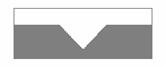

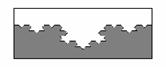
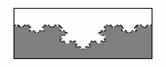
Fig. 3. Koch’s Triangular Curve.
In case of boiling we are interested in centres, and the characteristic size ![]() can be identified with
can be identified with ![]() . This
equation is applied now for N and
. This
equation is applied now for N and ![]() . Certainly with D = 2 we receive
again Labuntsov's formula (12) for centres density.
. Certainly with D = 2 we receive
again Labuntsov's formula (12) for centres density.
After simple substitutions we receive equation
(14) for the distance L between the centres:
![]() (14)
(14)
or, in view of the requirements of physical
dimension,
 (15)
(15)
where ![]() - linear scale for roughness,
- linear scale for roughness, ![]() -dimensionsless
coefficient. D is taken equal to 2 or
3 in the following calculations of the heat transfer coefficient.
-dimensionsless
coefficient. D is taken equal to 2 or
3 in the following calculations of the heat transfer coefficient.
But before that two examples of fractal
surfaces are shown (Feder,1988).
The first is known as Koch’s triangular curve
(Fig. 3). Each subsequent curve repeats the previous in smaller scale.
Probably, such structures will be formed at parallel grinding of a surface.
Here D equals 2.26.
The second example (Fig. 4) gives realistic
representation of an irregular rough surface. It is one of the first elementary
models by Mandelbrot.
Fig. 4. Realistic Representation of an Irregular Surface.
The “landscape” is created by the following
algorithm. The initial structure is a plateau with fixed height. Then, the
surface is received at repeated random superposition of such plateaus with
decreasing height. Here D equals 2.5.
RESULTS
Now the heat transfer coefficient at boiling is
calculated and the computer model is applied to boiling of water between 1 and
200 bar, as an example.
The calculation with the computer model was
conducted for two ways of evaluation of centres
density. Fractal dimension D is
taken: D = 2 (+, x , * in Fig.5 for 1 bar, 100 bar and 200 bar,
respectively) or D = 3 (§, w, Ÿ in Fig. 5 for 1 bar, 100 bar and 200 bar,
respectively). The constant Dist was
fitted to experiments at 1 bar.
The open symbols in Fig. 5 indicate the
experimental results for pool boiling of water at different pressures
(1 bar, 100 bar and 200 bar) on silver tube,
copper tube coated with nickel, copper tube coated with chrome and on stainless
steel tube (Golovin, Koltshugin,
Labuntsov (1963), (1965)).
So in case D
= 2, the results at 1 bar are described exactly due to fitting of constant Dist, but up to 200 bar the deviations
between the experiments and the computer calculation are significant (cf., for
example, open symbols on top of the diagram and asterisks for 200 bar).
With D = 3 and constant Dist fitted again to 1 bar results are in good agreement at all
pressures from 1 up to 200 bar (cf. open symbols and closed symbols in Fig. 5).
The results were compared also with Labuntsov’s (1972) approximate boiling theory which was an
initial item for our computer model.
The theoretical Labuntsov’s
(1972) equation
 (16)
(16)
is based on model according to which heat
transfer at advanced nucleate boiling is limited by a thin residual liquid
layer on the wall. The thickness of this layer is determined by intensive
liquid velocity pulsations created by growing bubbles. As
scales of such fluid movement are chosen speed of steam generation and distance
centre to centre. Equation (12) was used for the centres
density.
This theory is in good agreement with
experiments at low pressure by ![]() as an empirical constant. However at large
pressure the divergence is significant. Therefore Labuntsov
considered a multiplier b as the
empirical factor dependent from pressure:
as an empirical constant. However at large
pressure the divergence is significant. Therefore Labuntsov
considered a multiplier b as the
empirical factor dependent from pressure:
 (17)
(17)
In such form the Labuntsov’s
(1972) equation is used frequently in practice as a fitting curve for
experimental data.