Solving of algebraic equation and system
or
Van Gogh in Mathcad
(Translation into English with help by R.
Faucher – rfauch2001@yahoo.com)
(Another articles of Valery
Ochkov)
Valery Ochkov
Fig. 1. Search of roots of the
equation by means of symbolical mathematics Mathcad/Maple
Fig. 2. Numerical search
of a root of the equation
Fig. 3. "Picture" of roots
of function root at two arguments
Fig. 3a. “Picture” of roots of
function Find at one unknown
Fig. 4. "Picture" of roots
of the function root with 4 arguments
Fig. 5. Numerical search of roots of
system of two nonlinear algebraic equations
Fig. 6. "Picture" of roots
of the function Find (Mathcad 2000)
Fig. 6a. "Picture" of
roots of the function Find (Mathcad 2001i + Plots of System)
Fig. 7. «Landscape at Auveres
after the rain» by Vincent Van Gogh
Fig. 6a. A choice of a method of
search of roots of system of the algebraic equations
Рис. 7а. "Picture" of roots
of the function Find (Conjugate Gradient Method)
Рис. 7b. "Picture" of
roots of the function Find (Quasi-Newton Method)
Fig. 6b. "Picture" of
roots of the function Find (CTOL=10-15)
Рис. D1. Аналитический поиск
корней системы двух нелинейных алгебраических уравнений
First, about the
terms of the article
The
root of a function is a value of its argument, at which the function is equal
to zero[1].
The
root of an algebraic equation is a value of its unknown, at which the equation
becomes identity.
The
root of a system of algebraic equations are values of its unknowns at which the
equation which is included in system, we identity.
One of typical
tasks solved in Mathcad is a search of roots of the algebraic equations and
their systems: a finding of unknown values (unknowns in the case of one
equation), at which equation turns to identities. In Mathcad there is a wide
tooling (commands of the menu, functions and operators) for the numerical,
analytical and graphical solution of this task.
The basic
features of numerical search of roots of the nonlinear[2] algebraic equations and systems are
as follows:
1. One root from many existing ones is
determined. Which root will be found depends mainly on the first approximation
to the solution (guess values).
2. No root of the equation or system is
searched, and the value unknown (unknowns), at which deviation of the right and
left parts of the equations (discrepancy) does not exceed the previous number
given. In Mathcad, by default, it is equal 10-3 (the values of the system
variable TOL and CTOL[3]).
3. Work of functions root and Find
(namely these are built-in functions in Mathcad for the solution of a header
task of the article) has certain random and unpredictable characteristics, that
distinguishes them from other built-in functions Mathcad. The function sin, for
example, always gives out the "predicted" answer: to each element of
the set "the argument of function" corresponds to the quite certain
element of set "value of function". In the relation to functions root
and Find, such clearness is not present: these functions can return at all that
from them expect, or in general under abnormal condition to interrupt the work,
having asked the user to change some parameters of search and to repeat
account. The function Find, in general, is completely contextually dependent:
the value, which it returns, depends not only and not how many on values of its
arguments, and how near it is written. It can be considered (examined) as a
certain infringement of a principle of functional dependence underlying
mathematics.
We shall also
note features of analytical and graphical search of roots in Mathcad.
By analytical
search[4] the Mathcad system tries to find
all roots with absolute (analytical) accuracy. Because of it, the decision of
even the elementary tasks frequently comes to an end by failure(see fig. 1).
Fig. 1. Search of roots of the equation by
means of symbolical mathematics Mathcad/Maple
In a fig. 1 the analytical
(symbolic) search of roots y of the equations sin(x)/x = 0 and sin(x) = 0 is shown. Though at these equations of roots the
uncountable set, in the first case instead of a root is given out the message
on a mistake "No solution was found", and at simpler second equation sin(x) = 0 symbolical mathematics Mathcad are found by (with) a
unique(sole) root х = 0.
The Plot of Mathcad basically is used for verification
(check) of correctness of the decision and - or for specification of the data
for the first approximation by numerical search of roots. In fig. 1 (and fig. 2, seen lower) the plot
of function sin(x)/x, for example, is shown on a piece -10, 10 six times
(the fig. 1) crosses an axis x, but
on which symbolical mathematics Mathcad, nevertheless, has "broken".
The Mathcad built-in function root searches a root of
the equation by numerical methods. Since Mathcad 2000, the function root can
have not only two arguments (the combination of methods of
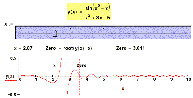
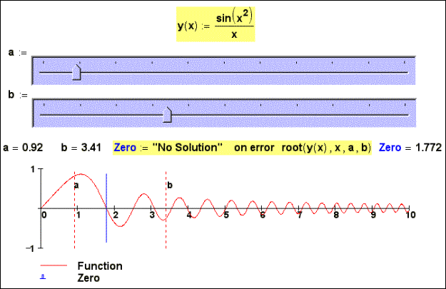
Fig. 2. Numerical
search of a root of the equation
But in the article the
Plots of Mathcad will be involved not in absolutely usual aspect – for
visualization of functions returning roots of the equations and systems and
having as arguments the values of the first approximation (guess values).
New opportunities not only for the analysis of those or other numerical methods
realized in Mathcad, but also for … of art creativity here open.
In a fig. 3 and the fig. 4 is shown, what roots of the equation sin(x)/x = 0 returns the function root
depending on values of the first approximation.
Fig. 3. "Picture" of roots of function root
at two arguments
The diagram in a fig. 3 is certain the
"portrait" of a method of Newton-secant, which essence is those.
Through two points (one of which is first approximation, and second recedes to
the right from new on distance TOL) will be carried out secant, which crossing with an
axis x gives a point of the second approximation. But previous values of the
function in a point of the first approximation are checked, that early: if it
is less TOL, the task is considered solved. If there is no – an
iteration proceed: secants will be carried out through new pairs points. Only
at the first approximation will be carried out, not secant, and actually
tangent (method of
From here we get to the clear diagram in fig. 3: when the value х on the module does not
exceed the value of system variable TOL (10-3), the
root is for one iteration (see the middle of fig. 3), and if it exceeds,
behind some iterations. Thus to foresee which root will be found, it is rather
difficult: the value of roots have scattered in a wide range (see left and
right edge(territory) of fig. 3).
For search of a root of the equation
it is possible to use also function Find, writing down before it not system,
but single equation (fig. 3a).
Fig. 3a. “Picture” of roots of function Find at
one unknown
In this case (fig. 3a) the character of points of the
first approximation near to critical points will be quite predicted: the
function Find is based not various updating gradient methods (see below) –
decision "rolled up" either to the left, or to the right. One is a
bad – function Find works on the order more slowly than the function root.
Fig. 4. "Picture" of roots of the function
root with 4 arguments
The function root,
returning a root of the equation sin(x)/x = 0 by method of haft division, as remarked earlier, has
not one, and two arguments. Hence, its visualization requires any more line (fig. 3 and fig. 3а), but a surface (fig. 4). Besides at the
formation of the function Rt the operator of processing of mistakes was used:
when the function root can not give out a root, the function Rt
returns the number 23 (number, it is more than 7 π – maximal root on a the
surface a-b). This number in a fig. 4 is "painted"
in white colour, the roots have "topographical" colouring: small
values of roots (-7 π) – dark blue colour (depth of ocean), and large (7
π) – brown (top of mountains). The intermediate roots are
"painted" in intermediate colours (light-blue, green, yellow). All
this is together similar to a mosaic marble floor or picture in style of cubism[5].
For the numerical decision of systems of the algebraic
equations as already was marked above, the function Find,
working in pair with a keyword Given is
intended built-in in Mathcad.
Fig. 5. Numerical search of roots of system of two
nonlinear algebraic equations
In a fig. 5 the work of function Find
under the decision of system of two nonlinear algebraic equations is shown: the
function Find returns this or that root depending on values of the first
approximation. It is also shown that at "unsuccessful" first
approximation (in a fig. 5 it, for example, beginning of coordinates) the work
of function Find interrupts by the message on a mistake and appeal to
the user to change parameters of search: the first approximation, values the
system variable TOL and/or CTOL. If the first approximation includes complex numbers,
the function Find can return a complex (imaginary) root – see fig. 5a, where our system is
written down in a vector kind, when the unknown systems are not separate scalar
variable (x, y, z etc), and elements of a vector x (x0, x1, x2 etc).
Fig. 5a. Numerical search of the
valid and imaginary roots of system of the algebraic equations which have been
written down in a vector kind
But we shall return to
four real roots of the system. In a fig. 6 surfaces x-y is painted in four colours depending on
what root from four existing (see fig. 5) was found at the first approximation taken in the
given "colour" area. «Blank spots» in a fig. 6 (and fig. 7a and fig. 7b too) are areas, the
search of roots from which was interrupted by the error-message.
Fig. 6. "Picture" of roots of the
function Find (Mathcad 2000)
Fig. 6a. "Picture" of roots of the function Find (Mathcad
2001i + Plots of System)
Mathcad-sheet
When the author has
shown fig. 6 to man knowledgeable in
fine art, he was told, that it was … «Landscape at Auveres after the rain» by
Vincent Van Gogh. The truth, this "artman" had not time (was in time)
put on glasses, and fig. 6was shown to him have issued. But at more detailed
comparison the similarity of colour scale and "invoices" (strip
ridge, range) figures was marked. Whether or not it is so, we will let our
readers will decide for themselves, having compared fig. 6 and fig. 7.
Fig. 7. «Landscape at Auveres after the
rain» by Vincent Van Gogh
But we shall leave in the party «the aesthetic party»
a fig. 6 and fig. 4 and we shall talk about
practical businesses.
In Mathcad three methods of the solution of systems of
algebraic equations are realized: the method Levenberg-Marquardt, the method of
the Conjugate Gradient, and methods of Quasi-Newton – see fig. 6a, where the local menu
appears after pressing of the right button of the mouse on the word Find).
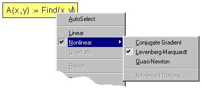
Fig. 6a. A choice of a method of search of roots of
system of the algebraic equations
So, the fig. 6 is "portrait" of the first method (it was
chosen by system Mathcad automatically for the decision of our system by
package Mathcad – see position AutoSelect in a fig. 6a), and the fig. 7a and fig. 7b is
"illustrations" of two other methods: Conjugate Gradient (fig 7a) and Quasi-Newton (fig. 7b).
Рис. 7а. "Picture" of roots of the
function Find (Conjugate Gradient Method)
Рис. 7b. "Picture" of roots of the
function Find (Quasi-Newton Method – try this Method on the MAS – http://twt.mpei.ac.ru/MAS/Worksheets/Newton_2.mcd)
It is simple to estimate
the relative area white patches in
a fig. 6,fig. 7a and fig. 7b and to give a certain
quantitative estimation of methods of the decision of systems of the nonlinear
algebraic equations realized in Mathcad. Here is how, for example, will look a
fig. 6 if to raise(increase) accuracy of accounts - to change values of
system variable TOL and CTOL from 10-3 (default) on 10-15 (fig. 6b).
Fig. 6b. "Picture" of roots of the
function Find (CTOL=10-15)
And figures (fig. 6, fig. 7a and fig. 7b) make certain triptych (three
"picturesque" cloths incorporated by one theme), which can be used
not only for an estimation of quality of those or other methods of search of
roots, but also for … of aesthetic pleasure. The author offers to the readers
to pick up other equations of system with other "picture" of roots.
In "picture” in a fig. 6 "beauty" has introduced lemniscate («twine by
colours») Bernoulli. But in mathematics still there are many other
"beautiful" curves, which can transfer "beauty" to figures
similar to a volume, to what is shown in a fig. 6.
Divertissement:
Рис. D1. Аналитический поиск корней системы двух нелинейных алгебраических уравнений
Рис. D2. Решение задачи из рассказа А.П. Чехова «Репетитор»: в системе уравнений одноименные, но разноцветные переменные
[1] More correctly to speak not about a root of function, and
about zero of function. But … see the article.
[2]Systems of the linear algebraic equations
is the special theme, with which in this article we shall not concern. Let's
note only that the linear equations and systems is a special case of
nonlinearity: the linear task is quite possible for deciding solving by
«nonlinear» tools, though it, to tell the truth, «chocking of nails by
microscope ». In Mathcad there are special tools for the solution of systems of
the linear equations which have been written down in the matrix form (function
lsolve, for example).
[3]In Mathcad up to the eighth version there was one system variable TOL (TOLerance, condescension
to an error). Then this variable has broken up on two TOL and СTOL. Now TOL "answers" for
work of functions root, Find, Minimize, Maximize and MinErr, and CTOL - for restrictions
(Constrains).
[4]The nucleus of
symbolical mathematics from a package Maple is built in Mathcad.
[5]We are
"selected" to second half of name of clause.